MLE estimation with noise parameter
Margarita Orlova
January 30, 2020
Last updated: 2020-02-05
Checks: 6 1
Knit directory: Thesis_single_RNA/
This reproducible R Markdown analysis was created with workflowr (version 1.5.0). The Checks tab describes the reproducibility checks that were applied when the results were created. The Past versions tab lists the development history.
Great! Since the R Markdown file has been committed to the Git repository, you know the exact version of the code that produced these results.
Great job! The global environment was empty. Objects defined in the global environment can affect the analysis in your R Markdown file in unknown ways. For reproduciblity it’s best to always run the code in an empty environment.
The command set.seed(20191113) was run prior to running the code in the R Markdown file. Setting a seed ensures that any results that rely on randomness, e.g. subsampling or permutations, are reproducible.
Great job! Recording the operating system, R version, and package versions is critical for reproducibility.
Nice! There were no cached chunks for this analysis, so you can be confident that you successfully produced the results during this run.
Using absolute paths to the files within your workflowr project makes it difficult for you and others to run your code on a different machine. Change the absolute path(s) below to the suggested relative path(s) to make your code more reproducible.
| absolute | relative |
|---|---|
| C:/Users/Moonkin/Documents/GitHub/Thesis_single_RNA/analysis/MLE.py | analysis/MLE.py |
| C:/Users/Moonkin/Documents/GitHub/Thesis_single_RNA/analysis/MLE_with_si.py | analysis/MLE_with_si.py |
Great! You are using Git for version control. Tracking code development and connecting the code version to the results is critical for reproducibility. The version displayed above was the version of the Git repository at the time these results were generated.
Note that you need to be careful to ensure that all relevant files for the analysis have been committed to Git prior to generating the results (you can use wflow_publish or wflow_git_commit). workflowr only checks the R Markdown file, but you know if there are other scripts or data files that it depends on. Below is the status of the Git repository when the results were generated:
Ignored files:
    Ignored:    .RData
    Ignored:    .Rhistory
    Ignored:    analysis/.RData
    Ignored:    analysis/.Rhistory

Unstaged changes:
    Modified:   Data_sim.Rmd
    Modified:   analysis/MLE_with_si.py
Note that any generated files, e.g. HTML, png, CSS, etc., are not included in this status report because it is ok for generated content to have uncommitted changes.
There are no past versions. Publish this analysis with wflow_publish() to start tracking its development.
In this section we have tried to implement \(s_i\) noise parameter as in Kim and Marioni paper.
The model is \(x|k_r,p \sim Poisson (s_ik_rp_i)\) where \(p|k_{on},k_{off}\sim Beta(k_{on},k_{off})\) and \(s_i\) is a total number of molecules which were sequenced in a cell, which captures noise (higher \(s_i\) means lower noise)
Warning: package 'reticulate' was built under R version 3.5.3Warning: package 'robustbase' was built under R version 3.5.1One dataset example
First, we generate one dataset and estimate MLE without noise variable:
k_on=as.numeric(0.1)
k_off=as.numeric(0.1)
kr=as.numeric(100)
n_cells=as.integer(100)
x=generate_data(k_on,k_off,kr,n_cells)
est=MaximumLikelihood(x)
est
[1] 0.1566934 0.1526440 100.3650009Then, we implement MLE calculation with \(s_i\) parameter included.
With \(s_i\)=1 we should receive the same estimators as without \(s_i\)
si=matrix(1, nrow = 100, ncol = 1)
x=generate_data_with_si(k_on,k_off,kr,n_cells,si)
est=MaximumLikelihood_with_si(x,si)
est
[1] 0.1032181 0.1157682 100.0291850With \(s_i\)=2, our \(k_r\) estimate drops twice, while \(k_{on}\) and \(k_{off}\) are not really affected by this change.
si=matrix(2, nrow = 100, ncol = 1)
x=generate_data_with_si(k_on,k_off,kr,n_cells,si)
est=MaximumLikelihood_with_si(x,si)
est
[1] 0.07899925 0.07777961 99.13065435We also try using different \(s_i\) values as this is what we will see in real data:
Multiple dataset results
Now we will also test model with \(s_i\) vs the model without it:
Initial MLE calculations:
[1] "true k_on is 0.1; k_on mean 0.101 k_on median 0.099"[1] "true k_off is 0.1; k_off mean 0.102 k_off median 0.1"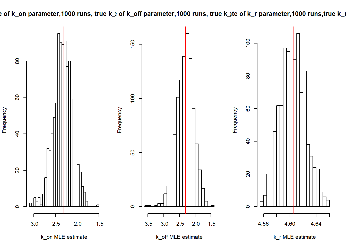
[1] "true k_r is 100; k_r mean 99.965 k_r median 99.925"MLE calculations with \(s_i\)=2 for all cells:
[1] "true k_on is 0.1; k_on mean 0.105 k_on median 0.1"[1] "true k_off is 0.1; k_off mean 0.118 k_off median 0.1"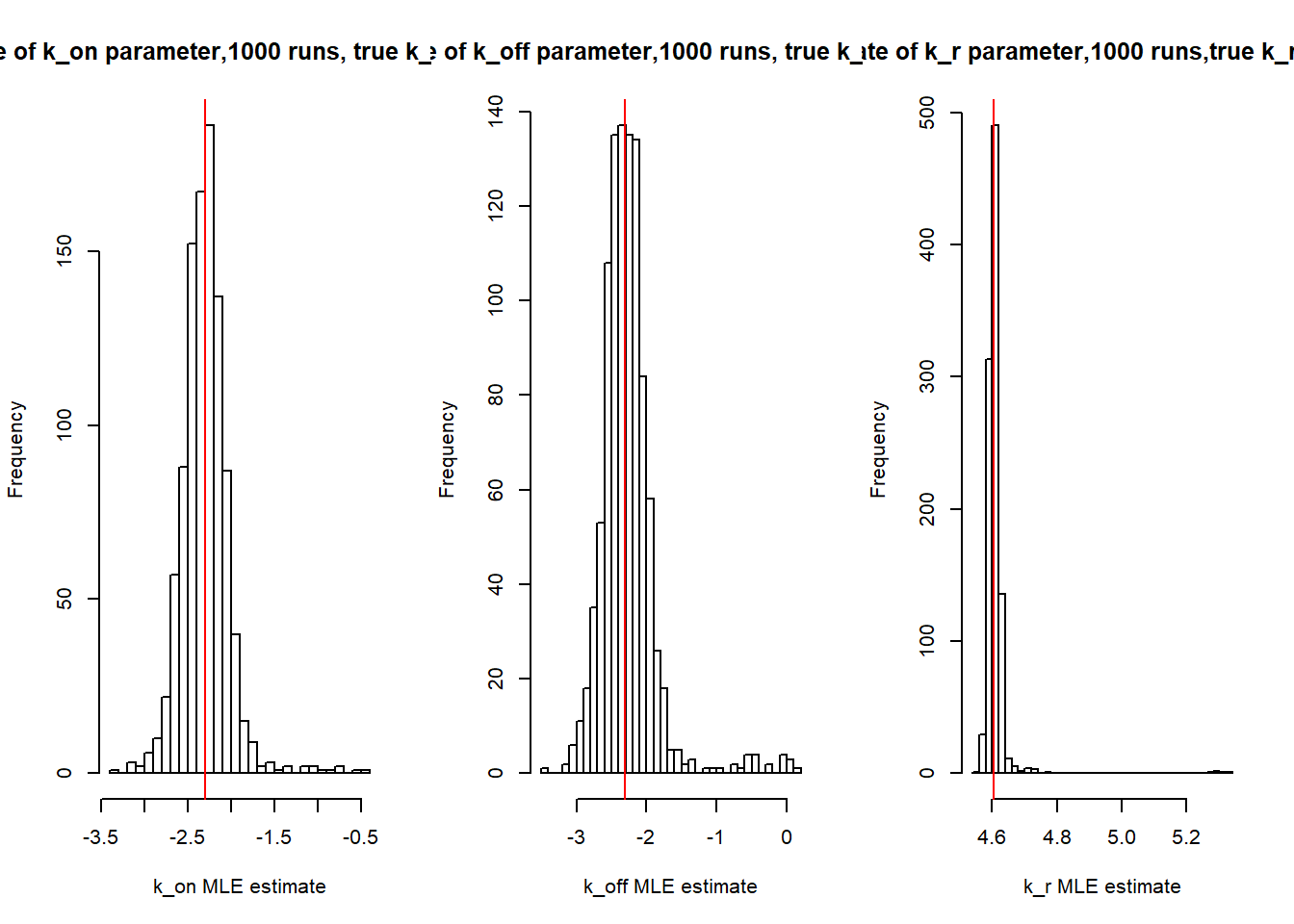
[1] "true k_r is 100; k_r mean 100.729 k_r median 100.056"Real data
We also estimate MLE with size parameter on the real data.
We use top gene with smallest p_beta parameter and obtain \(s_i\) for each cell from scqtl-annotation.txt.gz, mol_hs field
The MLE estimation without noise can be found here https://margareth2407.github.io/Thesis_single_RNA/Real_data_filter.html
Warning: package 'dplyr' was built under R version 3.5.3
Attaching package: 'dplyr'The following objects are masked from 'package:stats':
filter, lagThe following objects are masked from 'package:base':
intersect, setdiff, setequal, unionWarning: Column `gene` joining factors with different levels, coercing to
character vectorestimate_MLE_one_gene_with_si<-function(full_data,full_si){
data_ind<-substr(colnames(full_data),0,7)
data_ind<-data_ind[2:length(data_ind)]
est=matrix(, nrow = (length(unique(data_ind))-1), ncol = 3)
info=matrix(, nrow = (length(unique(data_ind))-1), ncol = 2)
iter=0
for (i in unique(data_ind)){
if (i=="NA18498"){
next}
iter=iter+1
x=full_data[ , grepl(i, names(full_data))]
si=data.frame(colnames(x))
colnames(si)<-c("id")
si<-left_join(si, full_si, by = "id")
si=data.matrix(si[,2])
x=t(data.matrix(x))
est[iter,]=MaximumLikelihood_with_si(x,si)
info[iter,1]=i
info[iter,2]=dim(x)[1]
}
return(list(est,info))
}options(warn=-1)
top_gene<-clean_data[1,]
results=estimate_MLE_one_gene_with_si(top_gene,full_cell_info)
est=results[[1]]
info=results[[2]]
par(mfrow=c(1,3))
hist(log(est[,1]),breaks=30, main="MLE estimate of k_on parameter, log scale", xlab="k_on MLE estimate")
hist(log(est[,2]),breaks=30, main="MLE estimate of k_off parameter, log scale", xlab="k_off MLE estimate")
hist(log(est[,3]),breaks=30, main="MLE estimate of k_r parameter, log scale", xlab="k_r MLE estimate")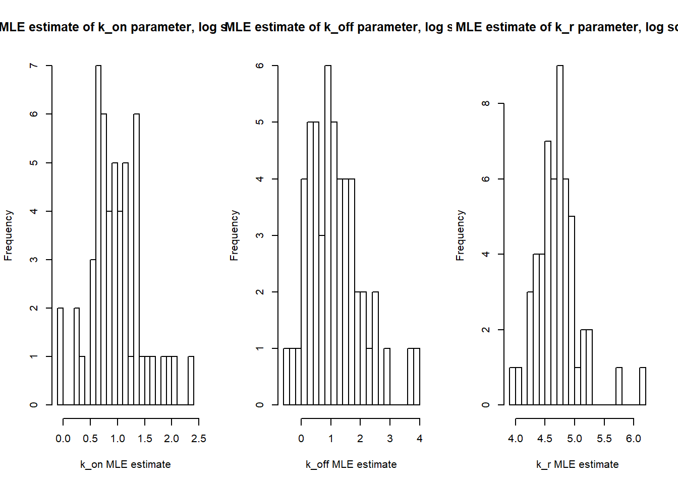
We can compare that with MLE estimation without size parameter
estimate_MLE_one_gene<-function(full_data){
  data_ind<-substr(colnames(full_data),0,7)
  data_ind<-data_ind[2:length(data_ind)]
  est=matrix(, nrow = (length(unique(data_ind))-1), ncol = 3)
  info=matrix(, nrow = (length(unique(data_ind))-1), ncol = 2)
  iter=0
for (i in unique(data_ind)){
  if (i=="NA18498"){
    next}
  iter=iter+1
  x=full_data[ , grepl(i, names(full_data))]
  x=t(data.matrix(x))
  est[iter,]=MaximumLikelihood(x)
  info[iter,1]=i
  info[iter,2]=dim(x)[1]}
return(list(est,info))}
top_gene<-clean_data[1,]
x1=estimate_MLE_one_gene(top_gene)
estimates1=x1[[1]]
info1=x1[[2]]
par(mfrow=c(1,3))
hist(log(estimates1[,1]), main="Distribution of k_on estimates", xlab="", ylab="Number of individuals")
hist(log(estimates1[,2]), main="Distribution of k_off estimates", xlab="", ylab="Number of individuals")
hist(log(estimates1[,3]), main="Distribution of k_r estimates", xlab="", ylab="Number of individuals")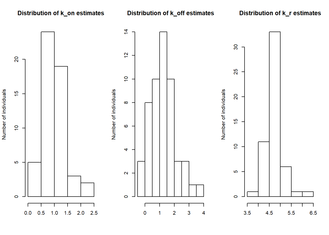
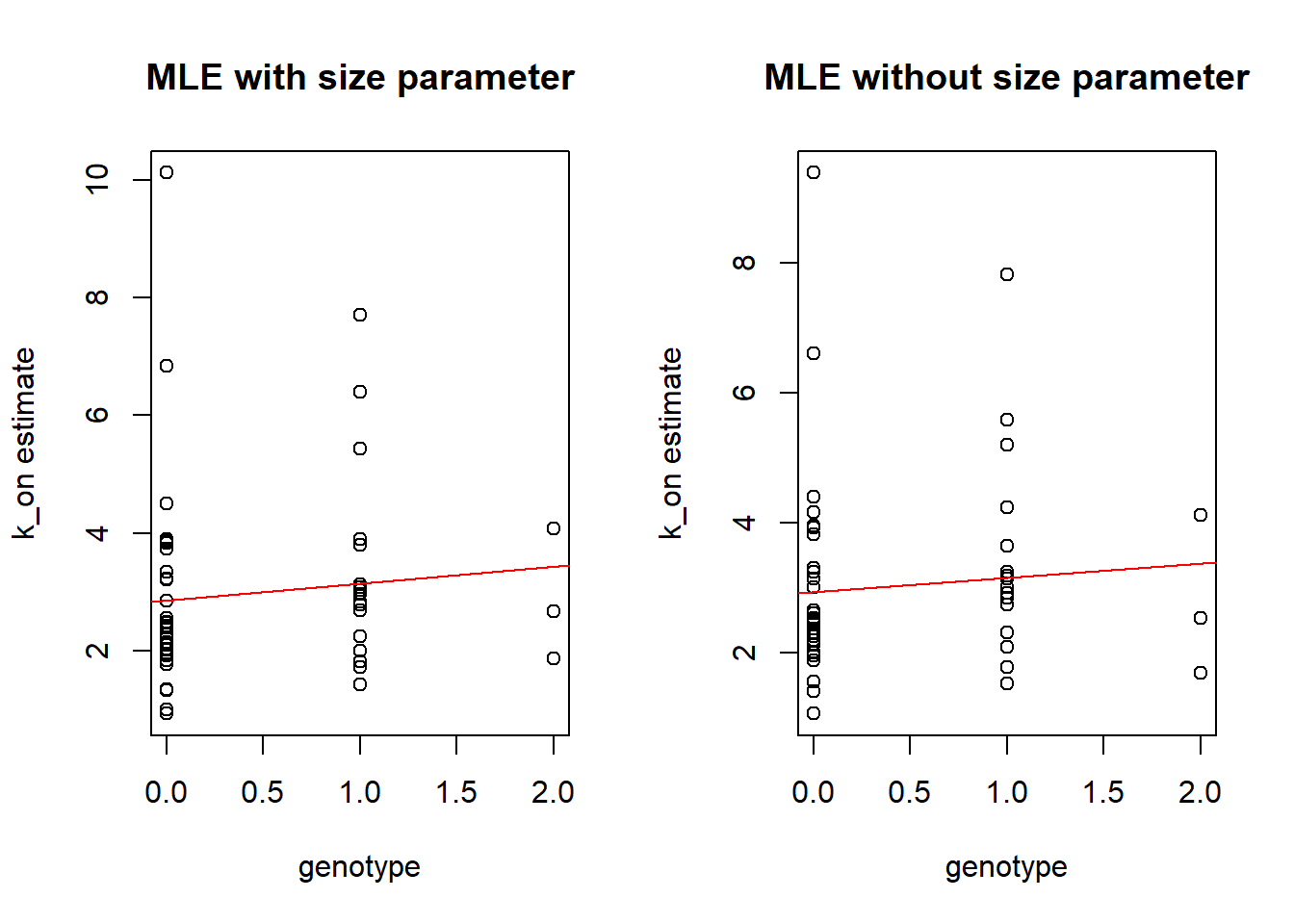
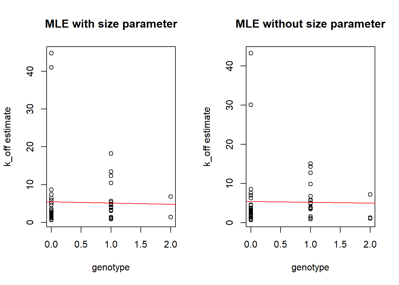
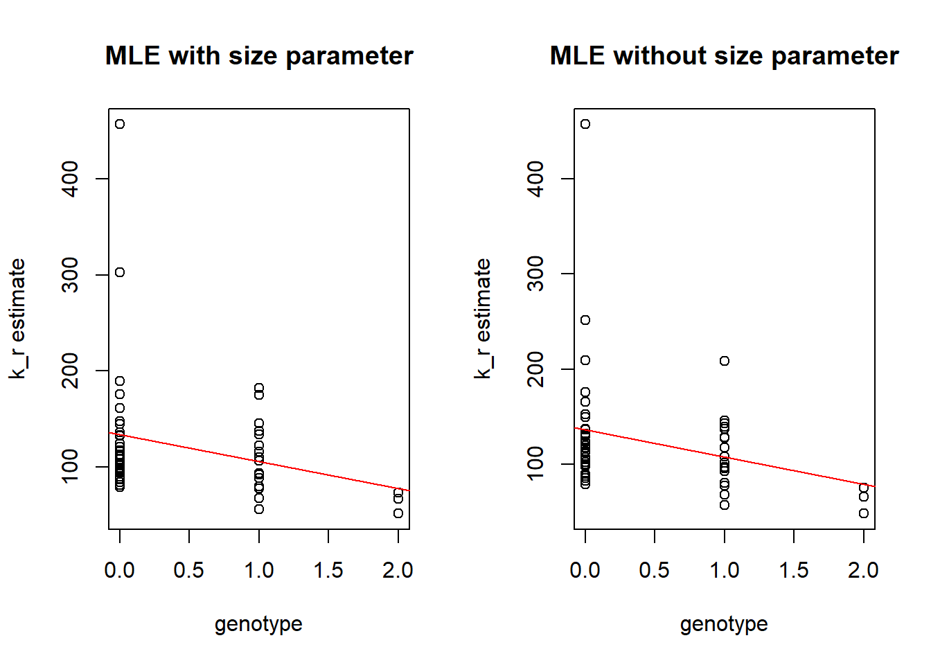
Boxplots by genotype
As in previous vignette we compare genotype to the estimated \(k_{on}\), \(k_{off}\) and \(k_{r}\) parameters.
Distribution for one individuals
par(mfrow=c(1,3))
na18501=top_gene[ , grepl("NA18501", names(top_gene))]
hist(data.matrix(na18501), xlab="Number of molecules", main="Distribution of protein expression") #Real data
beta=rbeta(200,est[24,1],est[24,2])
hist(beta, main="Beta distribution")
poisson=rpois(200,beta*est[24,3])
hist(poisson, xlab="Number of molecules",main="Poisson distribution")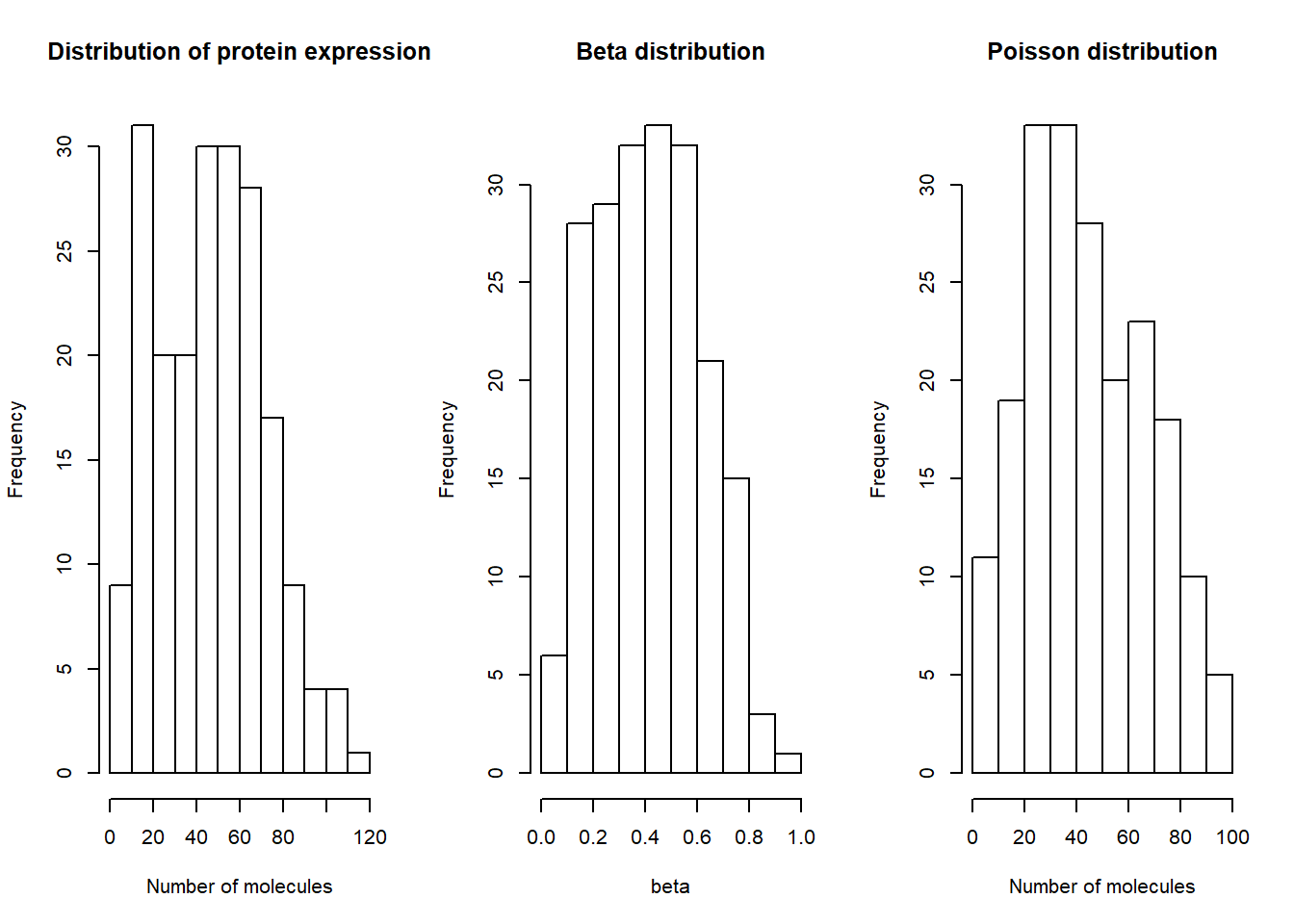
sessionInfo()R version 3.5.0 (2018-04-23)
Platform: x86_64-w64-mingw32/x64 (64-bit)
Running under: Windows 10 x64 (build 17763)
Matrix products: default
locale:
[1] LC_COLLATE=English_United States.1252
[2] LC_CTYPE=English_United States.1252
[3] LC_MONETARY=English_United States.1252
[4] LC_NUMERIC=C
[5] LC_TIME=English_United States.1252
attached base packages:
[1] stats graphics grDevices utils datasets methods base
other attached packages:
[1] dplyr_0.8.3 robustbase_0.93-3 reticulate_1.13
loaded via a namespace (and not attached):
[1] Rcpp_1.0.2 knitr_1.20 magrittr_1.5 workflowr_1.5.0
[5] tidyselect_0.2.5 lattice_0.20-38 R6_2.3.0 rlang_0.4.2
[9] stringr_1.3.1 highr_0.7 tools_3.5.0 grid_3.5.0
[13] git2r_0.26.1 htmltools_0.3.6 assertthat_0.2.0 yaml_2.2.0
[17] rprojroot_1.3-2 digest_0.6.17 tibble_2.1.3 crayon_1.3.4
[21] Matrix_1.2-14 purrr_0.2.5 later_0.8.0 fs_1.3.1
[25] promises_1.0.1 glue_1.3.0 evaluate_0.11 rmarkdown_1.10
[29] stringi_1.1.7 pillar_1.4.2 DEoptimR_1.0-8 compiler_3.5.0
[33] backports_1.1.2 jsonlite_1.5 httpuv_1.5.1 pkgconfig_2.0.2