MLE
Margarita Orlova
November 15, 2019
Last updated: 2020-02-01
Checks: 6 1
Knit directory: Thesis_single_RNA/
This reproducible R Markdown analysis was created with workflowr (version 1.5.0). The Checks tab describes the reproducibility checks that were applied when the results were created. The Past versions tab lists the development history.
Great! Since the R Markdown file has been committed to the Git repository, you know the exact version of the code that produced these results.
Great job! The global environment was empty. Objects defined in the global environment can affect the analysis in your R Markdown file in unknown ways. For reproduciblity it’s best to always run the code in an empty environment.
The command set.seed(20191113) was run prior to running the code in the R Markdown file. Setting a seed ensures that any results that rely on randomness, e.g. subsampling or permutations, are reproducible.
Great job! Recording the operating system, R version, and package versions is critical for reproducibility.
Nice! There were no cached chunks for this analysis, so you can be confident that you successfully produced the results during this run.
Using absolute paths to the files within your workflowr project makes it difficult for you and others to run your code on a different machine. Change the absolute path(s) below to the suggested relative path(s) to make your code more reproducible.
| absolute | relative |
|---|---|
| C:/Users/Moonkin/Documents/GitHub/Thesis_single_RNA/analysis/MLE.py | analysis/MLE.py |
Great! You are using Git for version control. Tracking code development and connecting the code version to the results is critical for reproducibility. The version displayed above was the version of the Git repository at the time these results were generated.
Note that you need to be careful to ensure that all relevant files for the analysis have been committed to Git prior to generating the results (you can use wflow_publish or wflow_git_commit). workflowr only checks the R Markdown file, but you know if there are other scripts or data files that it depends on. Below is the status of the Git repository when the results were generated:
Ignored files:
    Ignored:    .RData
    Ignored:    .Rhistory
    Ignored:    analysis/.RData
    Ignored:    analysis/.Rhistory

Unstaged changes:
    Modified:   Data_sim.Rmd
    Deleted:    analysis/MLE_estimation_with_noise_parameter.Rmd
    Deleted:    analysis/MLE_variability_by_sample_size.Rmd
    Deleted:    analysis/Real_data_filter.Rmd
Note that any generated files, e.g. HTML, png, CSS, etc., are not included in this status report because it is ok for generated content to have uncommitted changes.
There are no past versions. Publish this analysis with wflow_publish() to start tracking its development.
MLE estimates and sampling variability
In this section we infer parameter estimates by maximum likelihood and estimate sampling variability of MLE.
As explained in previous data simulation section, mRNA gene expression can be modelled as three or four parameter model.
For three-parameter model probability distribution is:
\(P(X\leq x) = \int_0^{1} P(X\leq x|k_r*p)f(p)dp=\frac{1}{B(k_{on},k_{off})}\int_0^{1} P(X\leq x|k_r*p)p^{k_{on}-1}(1-p)^{k_{off}-1}dp\)
Using \(t=2p-1\), \(p=\frac{t+1}{2}\) and \(dt=2dp\) we have
\(\frac{1}{B(k_{on},k_{off})}\frac{1}{2^{k_{on}+k_{off}-1}}\int_{-1}^{1} P(X\leq x|\frac{k_r(t+1)}{2})(1+t)^{k_{on}-1}(1-t)^{k_{off}-1}\), the integral can be computed with the use of Gauss-Jacobi quadrature method.
And as we discussed previously, \(BetaPoisson(x|k_{on},k_{off},k_r,d) = BetaPoisson(\frac{x}{d}|k_{on},k_{off},k_r)\), so same applies to the probability distribution of four-parameter model.
Using pdf of the model we can calculate log-likelihood for the data \(logL(k_{on},k_{off},k_{r},d)=\sum_x n(x) log(p(\frac{x}{d}|k_{on},k_{off},k_{r}))\), where \(n(x)\) is the number of cells with mRNA expression level equal to x.
To optimize the computations, we will choose initial values using method of moments.
E(X) and Var(X) can be estimated from the data directly
\(Var(X|k_r*p)=E(X|k_r*p)=k_r*p\) as mean and variance of Poisson distribution
\(E(X)=E(E(X|k_r*p))=k_r*\frac{k_{on}}{k_{on}+k_{off}}\) by Tower Law
\(Var(X)=E(Var(X|k_r*p))+Var(E(X|k_r*p))=E(k_r*p) + Var(k_r*p) = k_r\frac{k_{on}}{k_{on}+k_{off}} + k_r^2\frac{k_{on}*k_{off}}{(k_{on}+k_{off})^2(k_{on}+k_{off}+1)}\) by law of total variance.
From that we can estimate \(k_{on}=\frac{E(X)}{k_r}(\frac{E(X)(k_r-E(X))}{Var(X)-E(X)}-1)\) and \(k_{off}=k_{on}*\frac{k_r-E(X)}{E(X)}\)
d is estimated as 0.1*median(X), if this value is less then 1.0 and 1.0 otherwise. After we choose d, we also scale data prior to other parameter initialization. Initial estimate of \(k_r\) is chosen to be max(X).
Now we will implement the method above, using code provided by Larsson et al. publication. Since the original code is in python, we have to source it from MLE.py script, generate 1000 datasets with same \(k_{on}\),\(k_{off}\) and \(k_r\) and get the point estimates. We repeat this process 4 times with different \(k_{on}\),\(k_{off}\) scenarios.
Warning: package 'reticulate' was built under R version 3.5.3Warning: package 'robustbase' was built under R version 3.5.1I) Small \(k_{on}\) and \(k_{off}\) case:
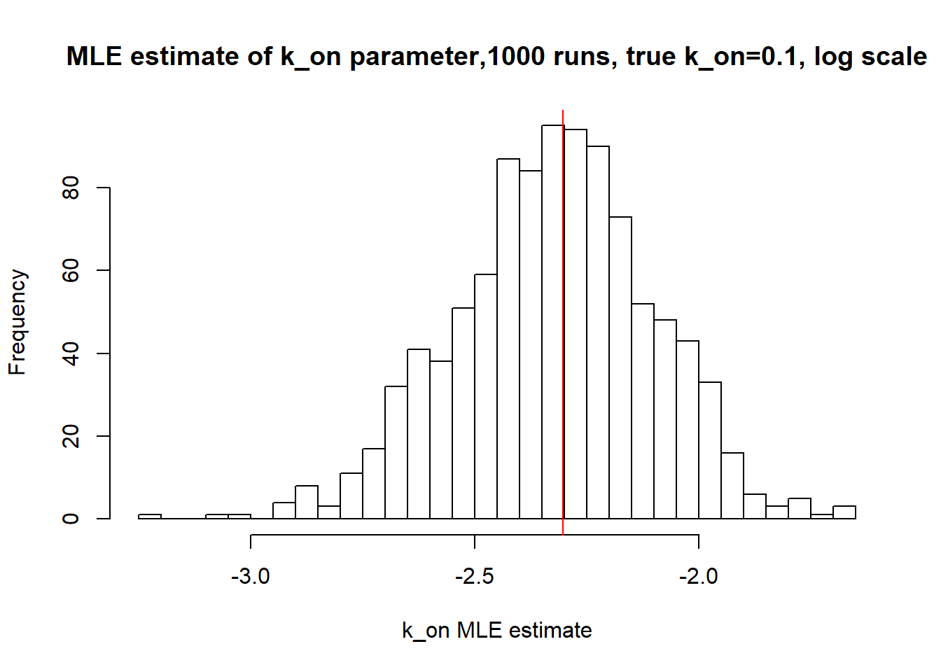
[1] "true k_on is 0.1; k_on mean 0.1 k_on median 0.098"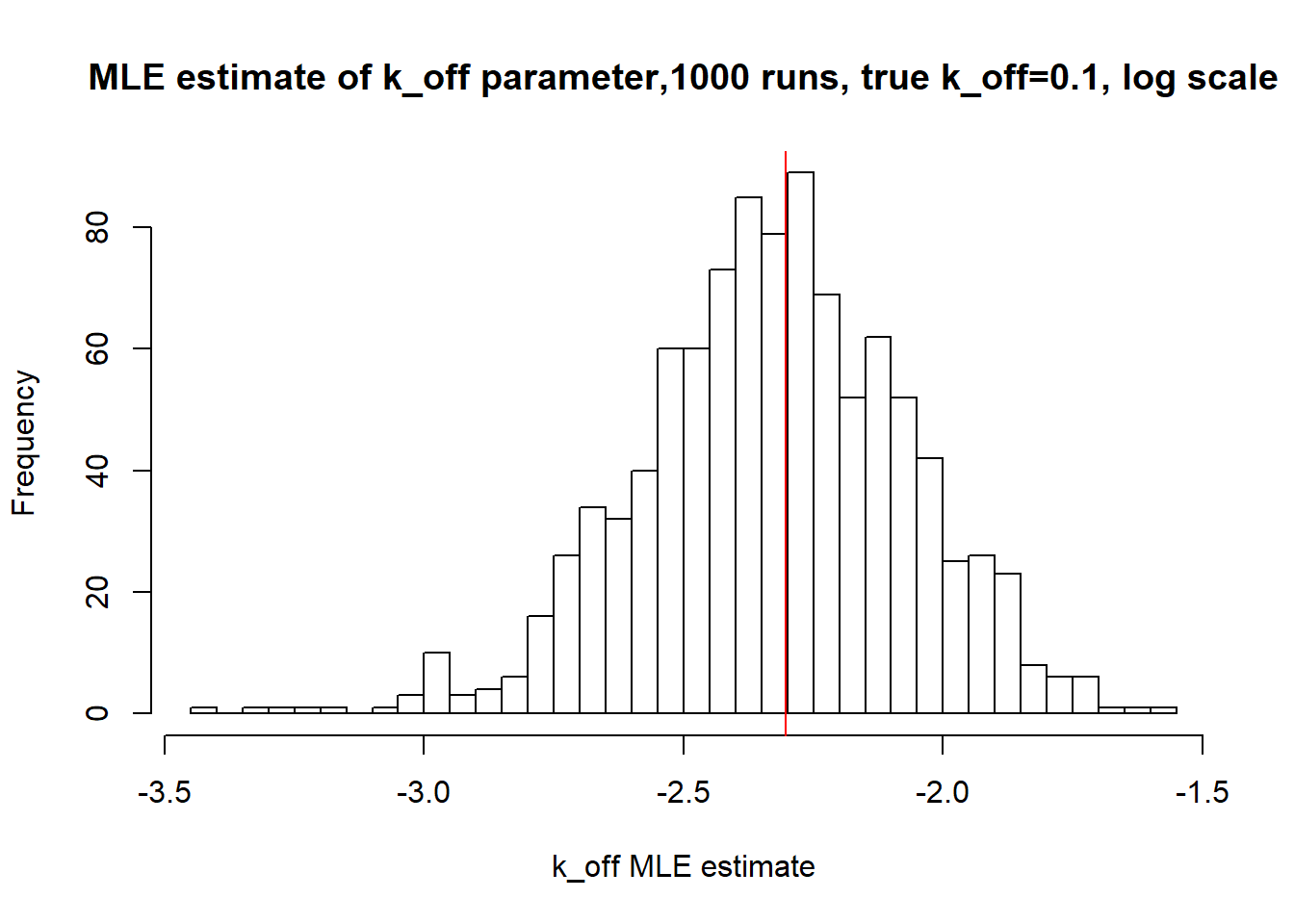
[1] "true k_off is 0.1; k_off mean 0.101 k_off median 0.098"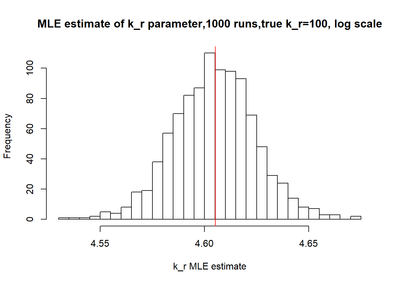
[1] "true k_r is 100; k_r mean 99.98 k_r median 99.959"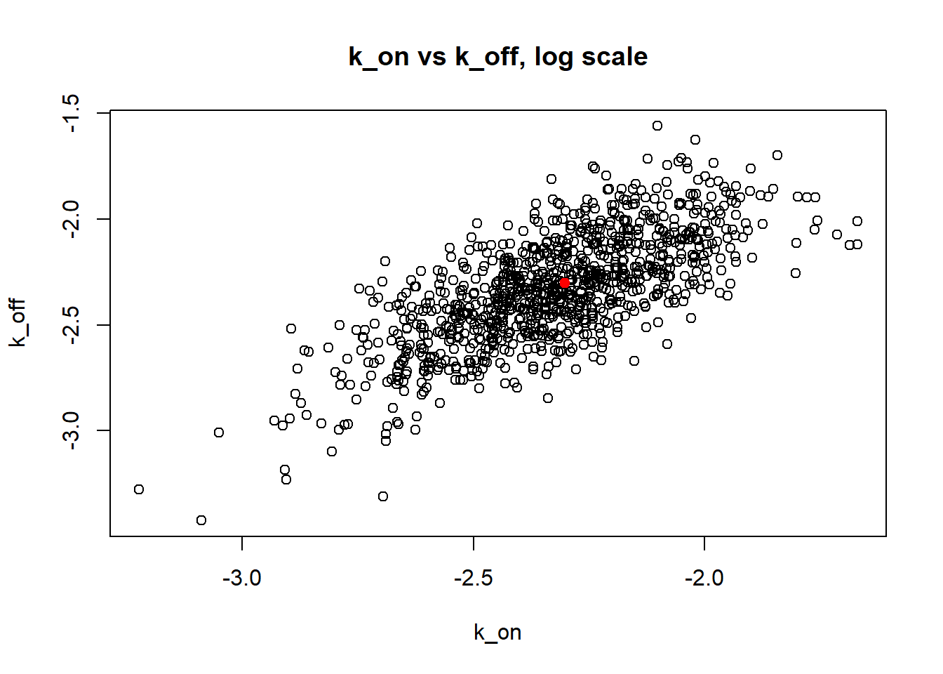
Small \(k_{on}\) and \(k_{off}\) leads to bimodal distribution where population of cells with high expression level is visibly separated from population of cells without expression. Such separation allows us to identify parameters very clearly and we will see more proofs of that in a future materials. Notice how both mean and median of the MLE estimates are close to the true value.
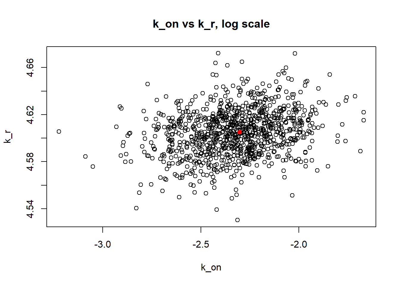
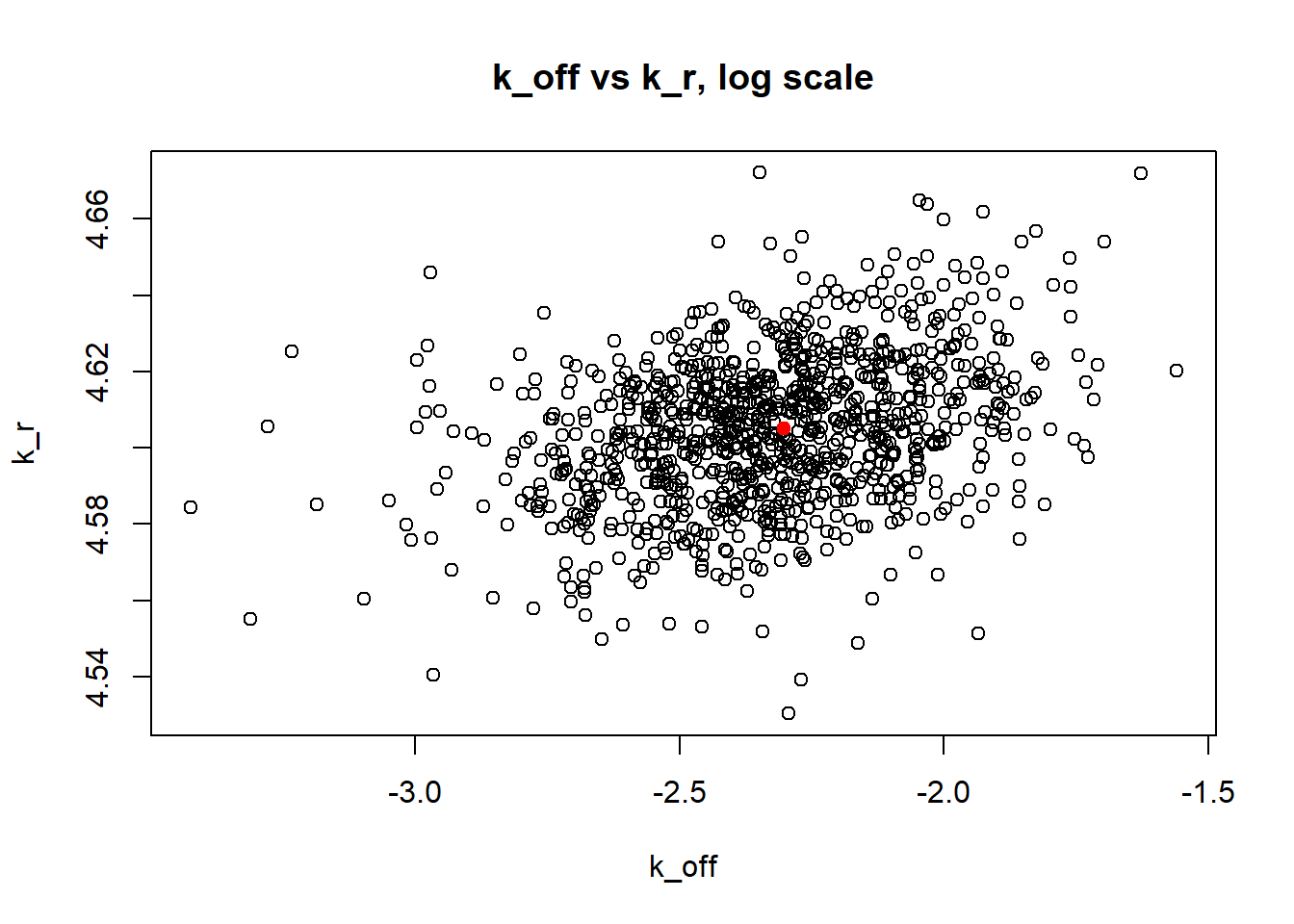
II) Large \(k_{on}\) and \(k_{off}\) case:
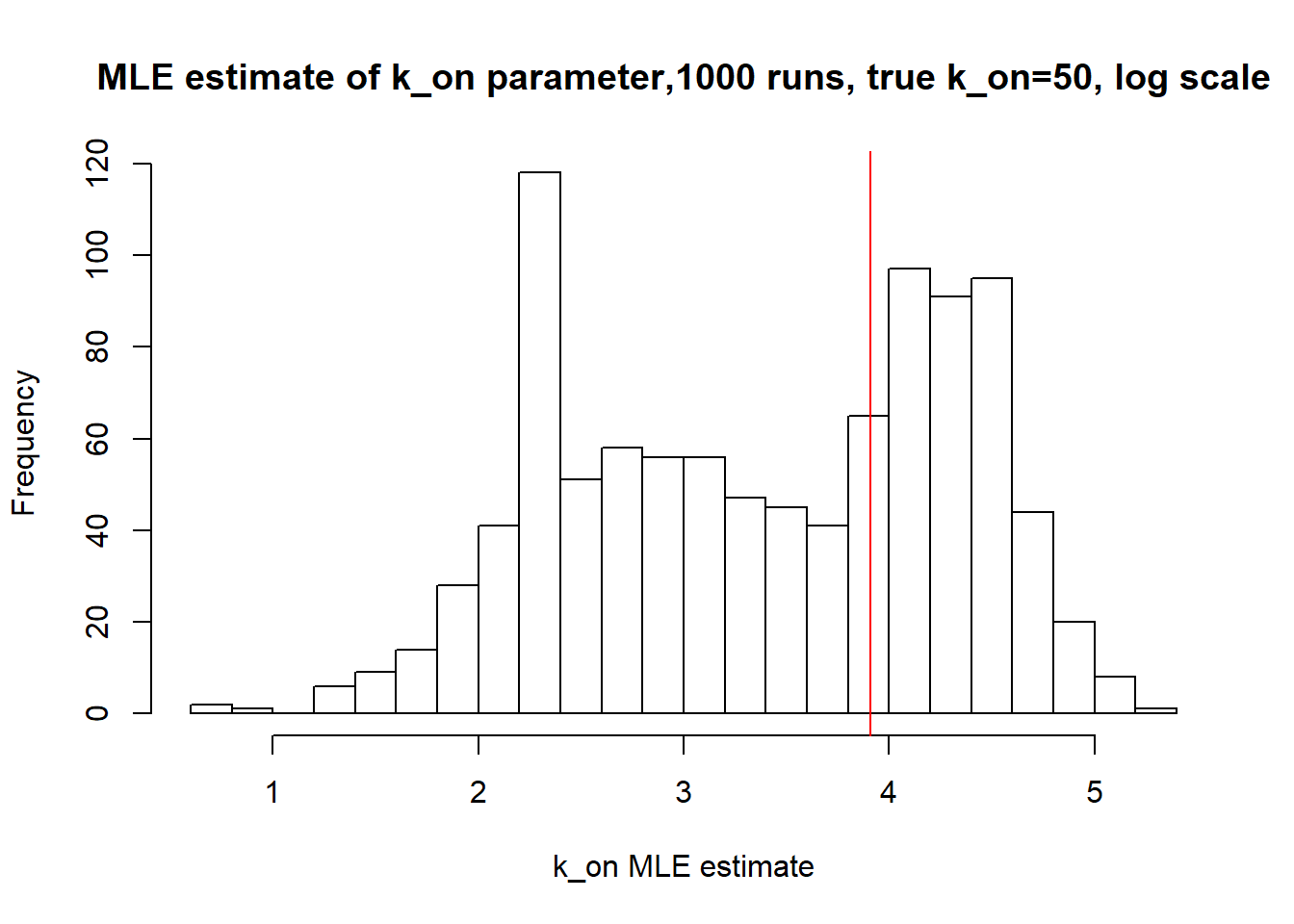
[1] "true k_on is 50; k_on mean 43.69 k_on median 30.898"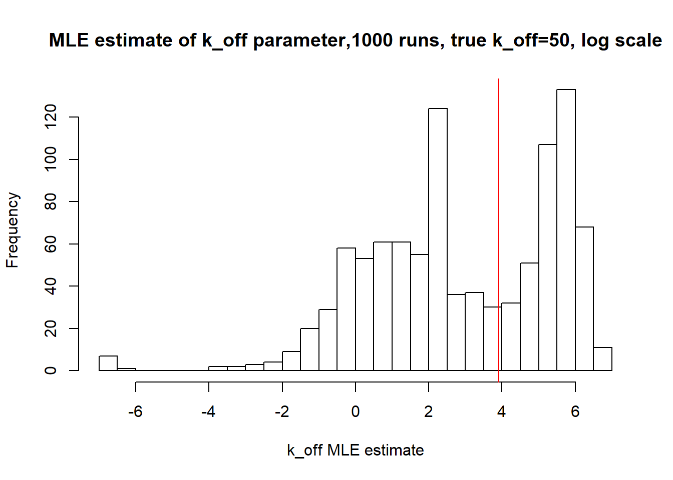
[1] "true k_off is 50; k_off mean 117.465 k_off median 14.569"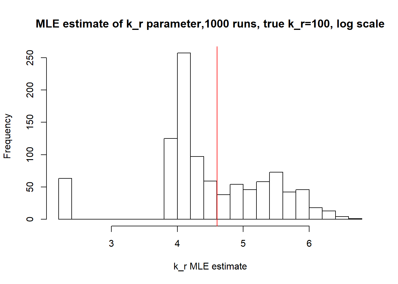
[1] "true k_r is 100; k_r mean 131.413 k_r median 72.744"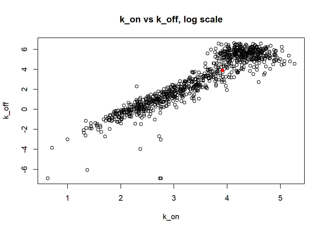
Large \(k_{on}\) and \(k_{off}\) case lead to Poisson or negative binomial distribution which means big population of highly expressed cells and small population of non-expressed cells. If cell quickly shift between active and non-active states, we cannot distiguish that from cell being constantly in active state which leads to unidentifiable solution. And indeed if we take a look on MLE estimates histogramms, means and medians we can observe that estimated parameters are not close to the true value in majority of cases.
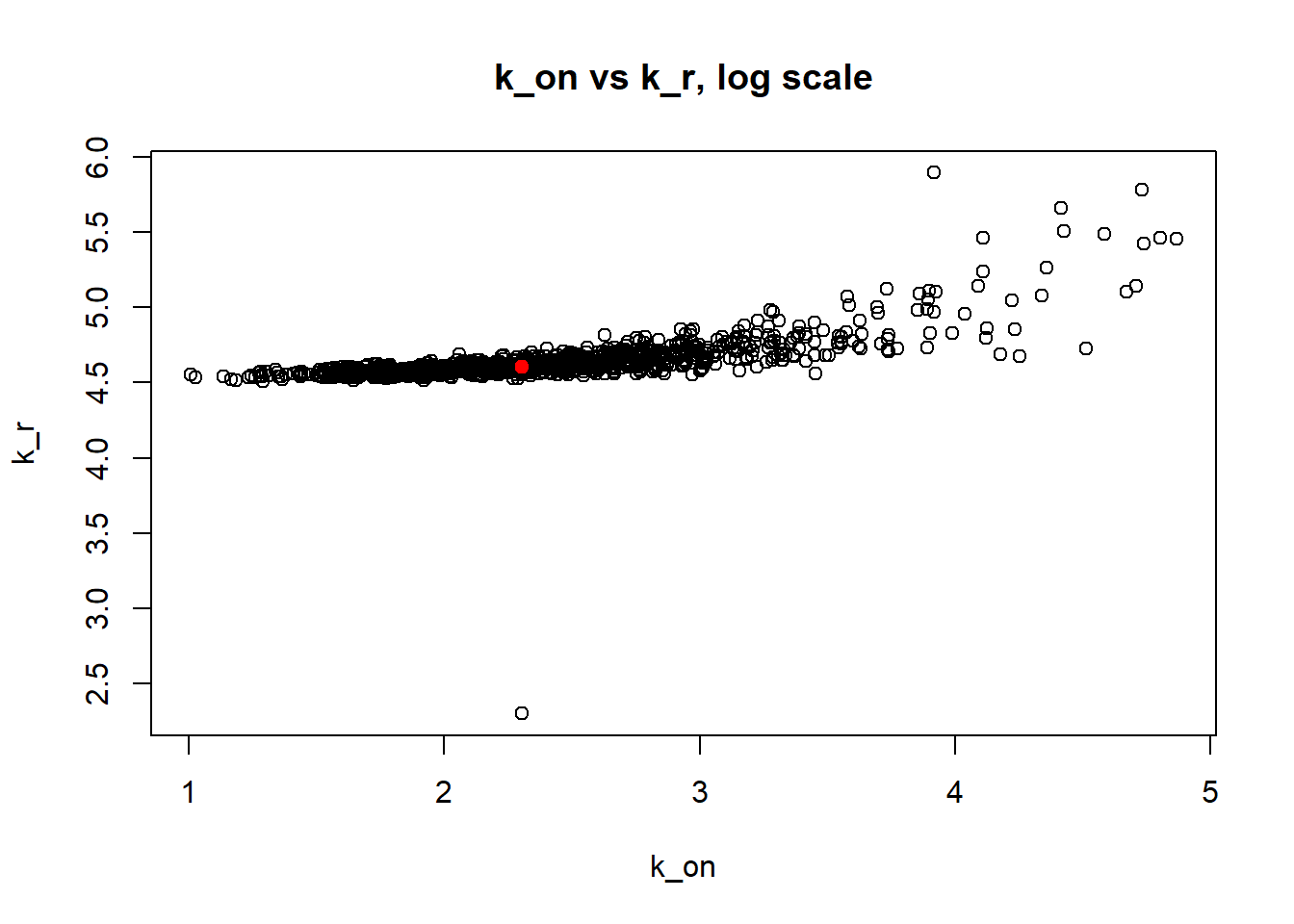
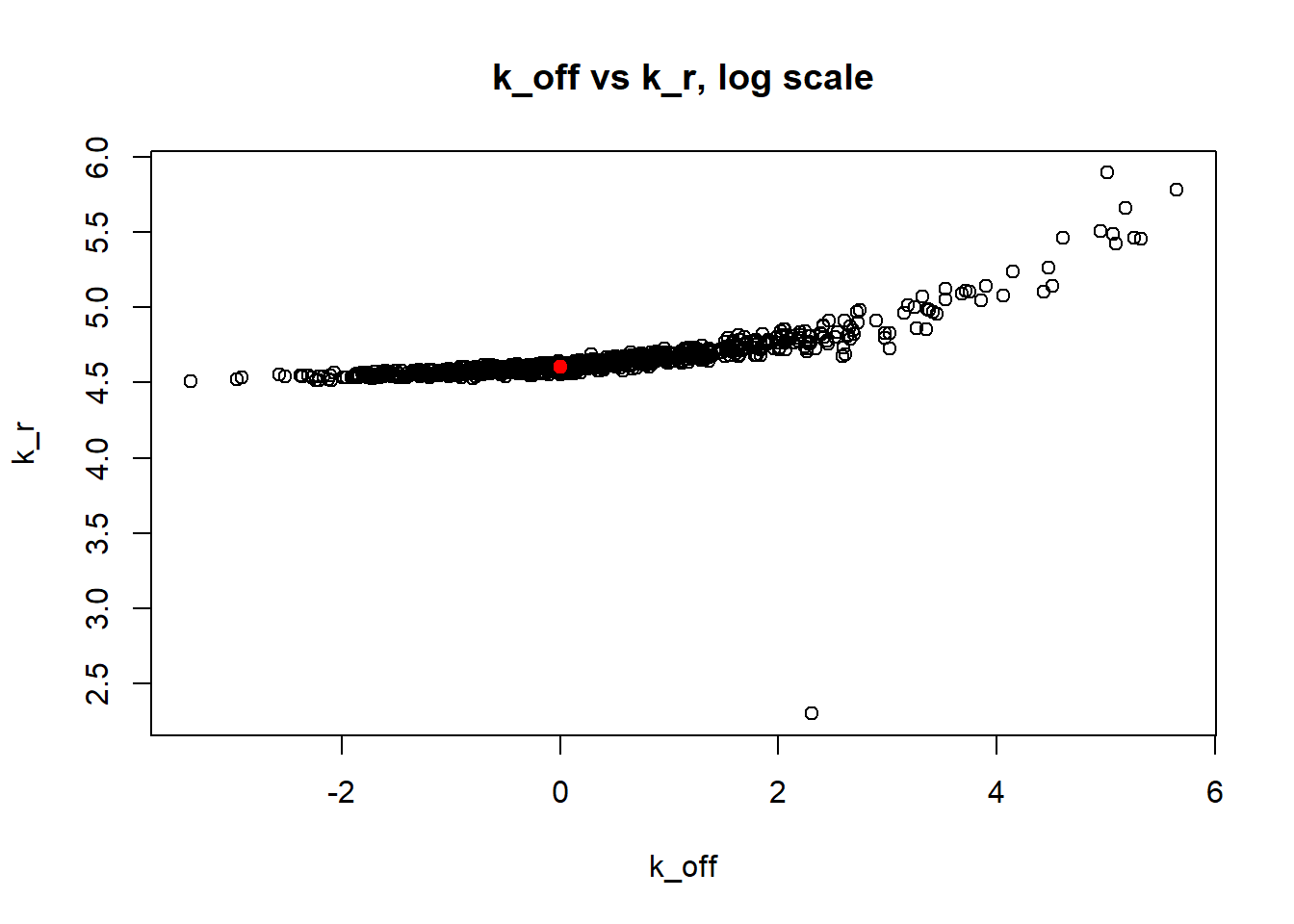
III) Large value of \(k_{off}\) and small \(k_{on}\) case:
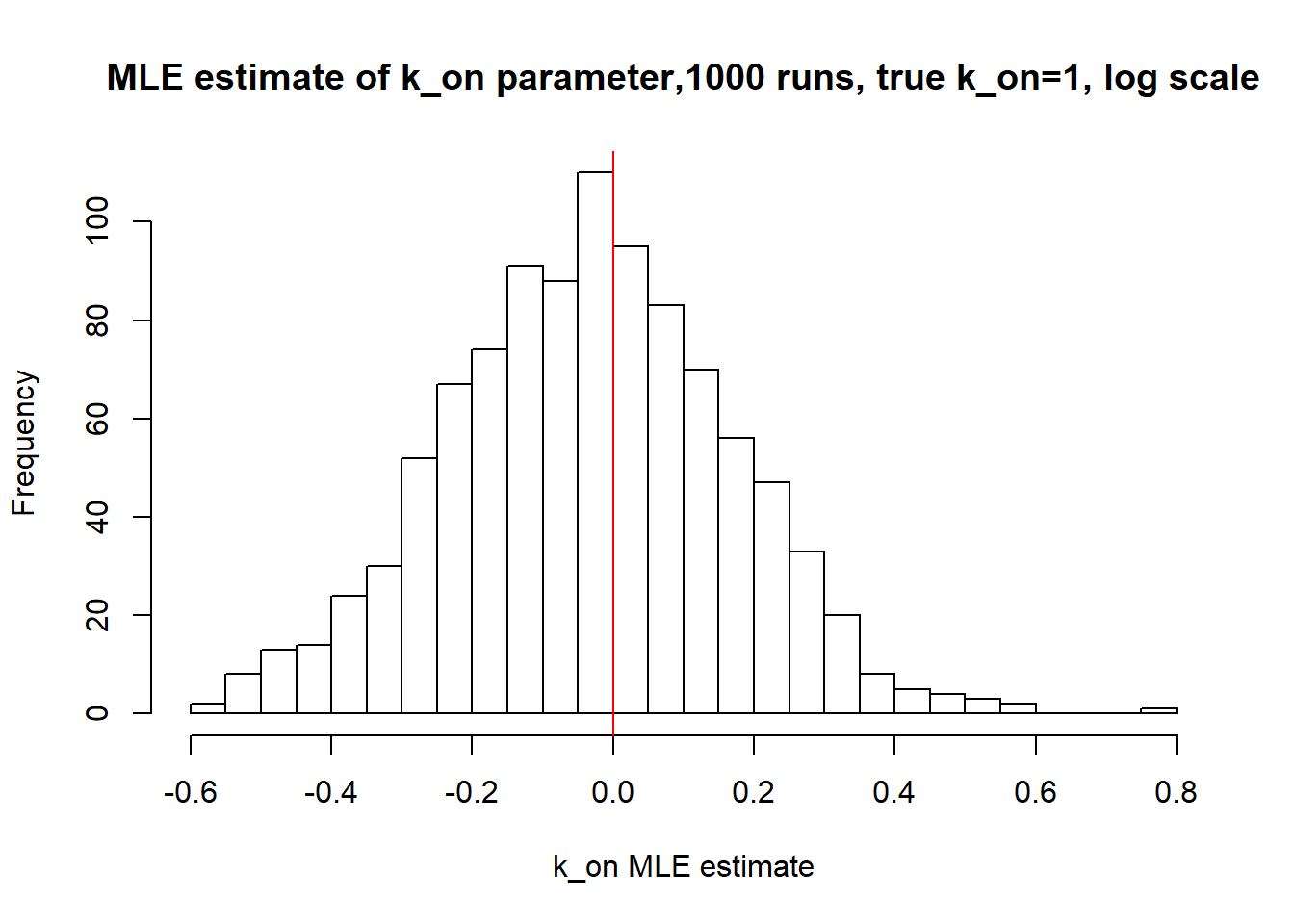
[1] "true k_on is 1; k_on mean 0.985 k_on median 0.969"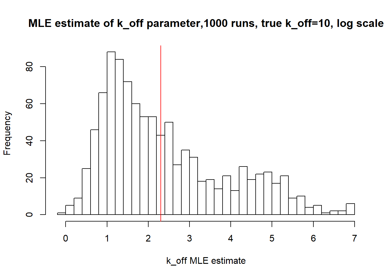
[1] "true k_off is 10; k_off mean 42.802 k_off median 7.055"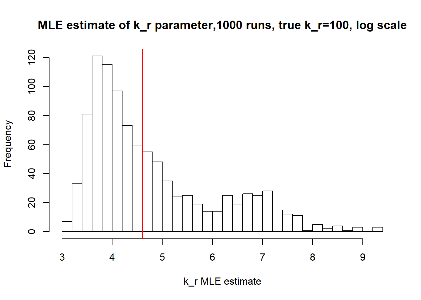
[1] "true k_r is 100; k_r mean 357.281 k_r median 73.906"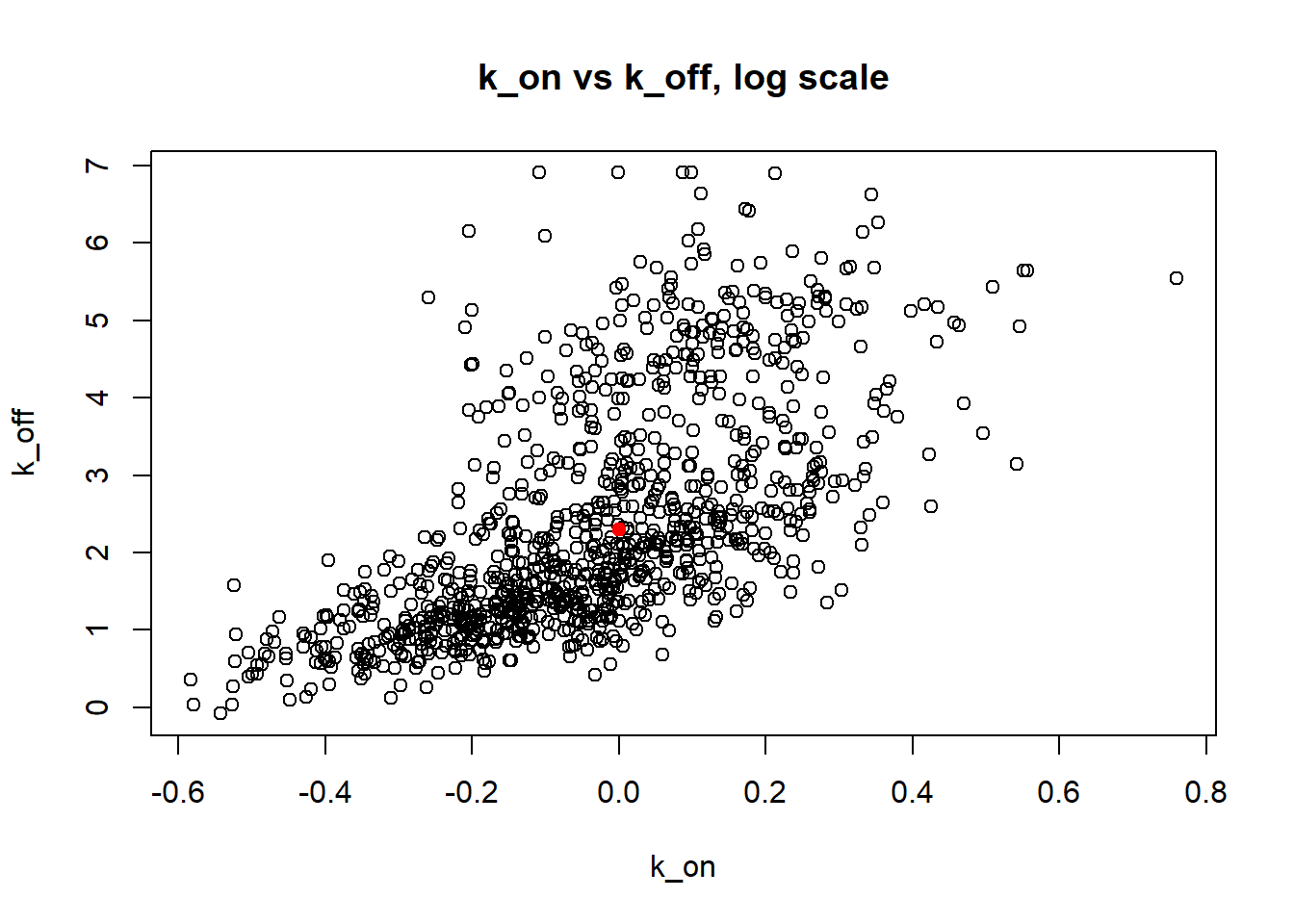
Large value if \(k_{off}\) and small \(k_{on}\) scenario results in majority of cells having zero or low expression levels. MLE method estimates \(k_{on}\) accurately by both mean and median while \(k_{off}\) and \(k_{r}\) are unidentifiable.
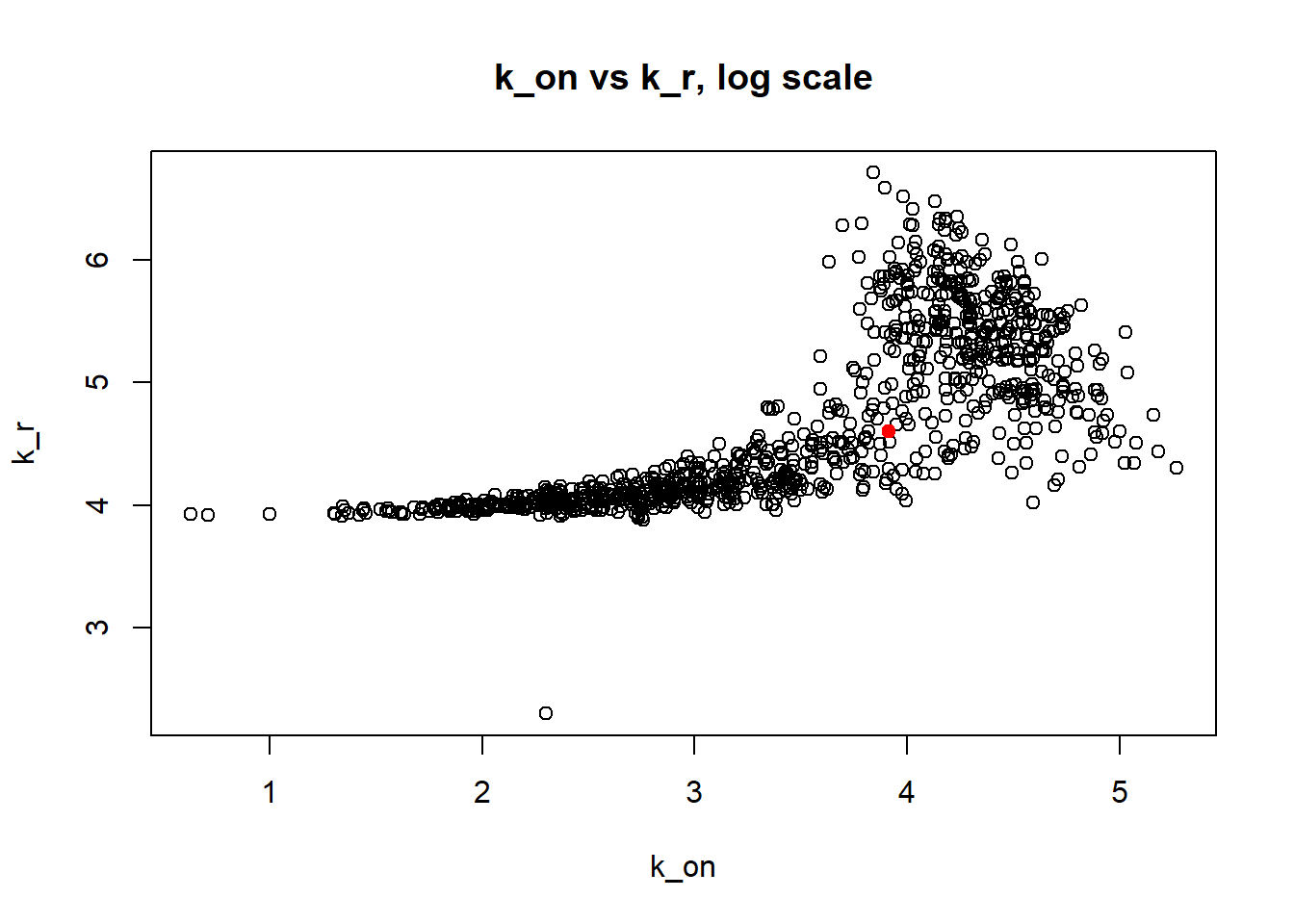
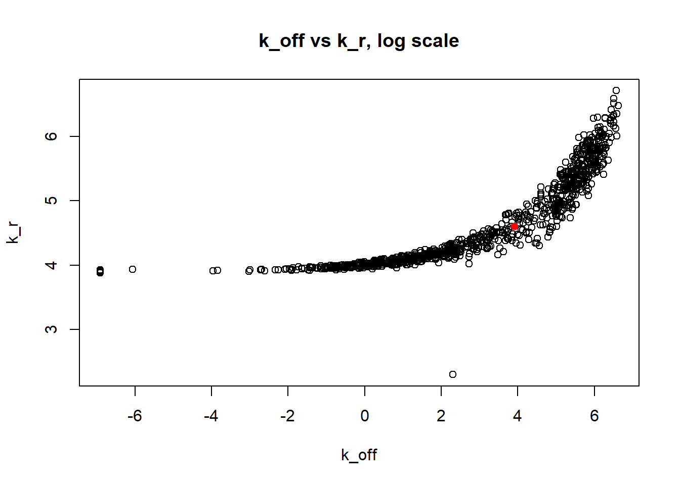
IV) Small value of \(k_{off}\) and big \(k_{on}\)
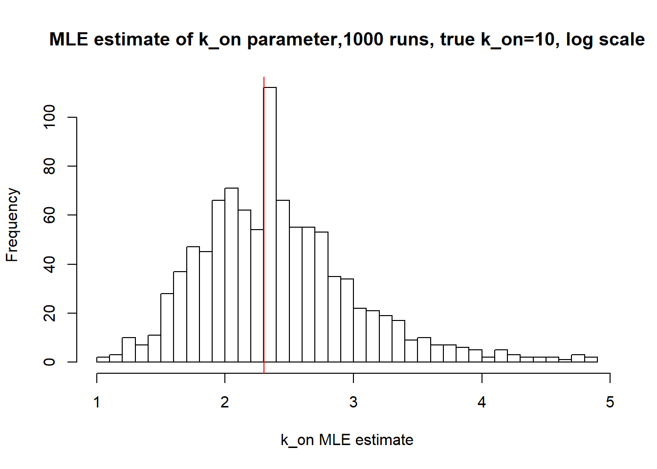
[1] "true k_on is 10; k_on mean 14.094 k_on median 10.073"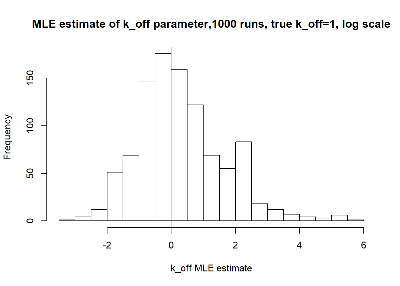
[1] "true k_off is 1; k_off mean 4.905 k_off median 1.155"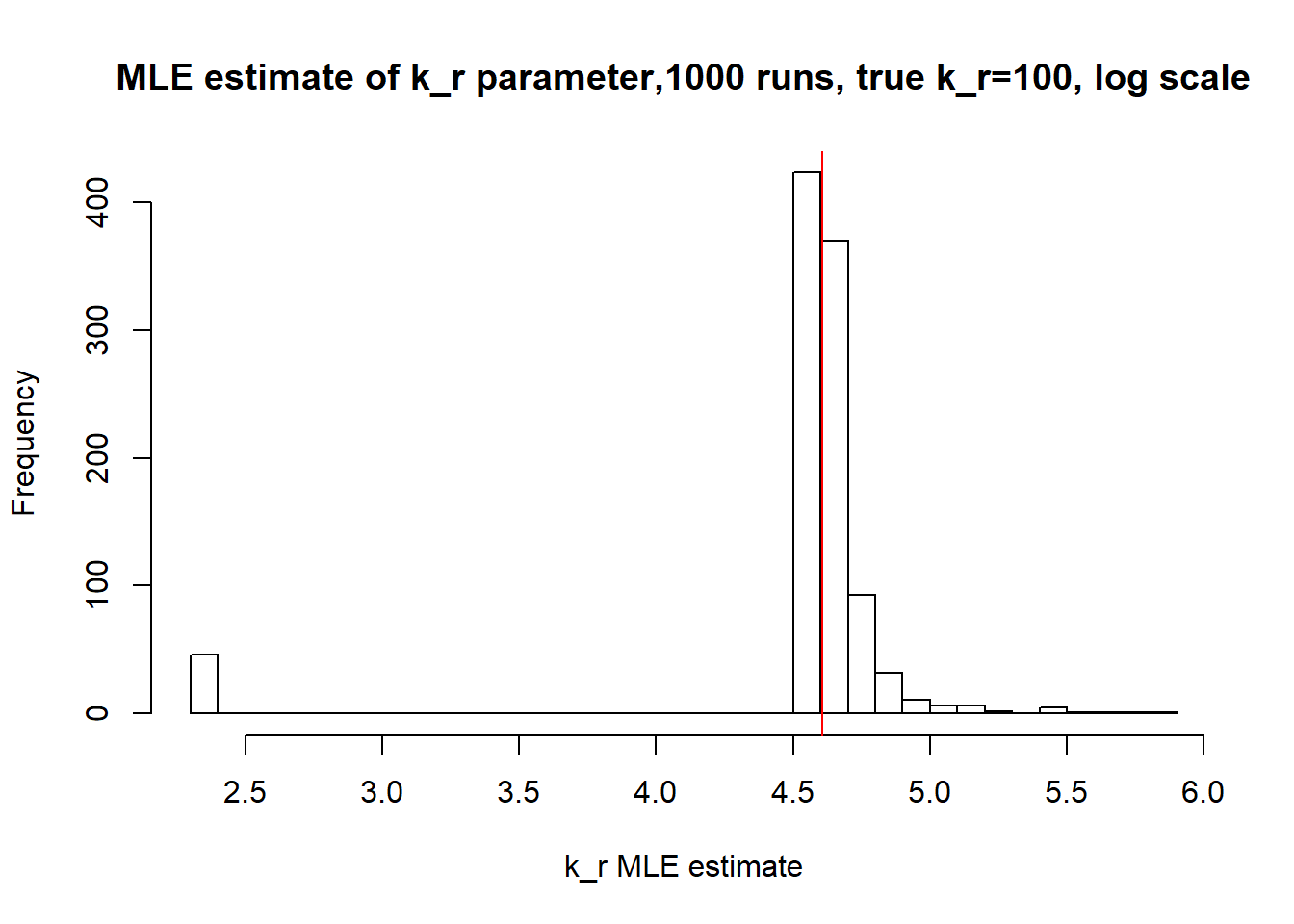
[1] "true k_r is 100; k_r mean 100.73 k_r median 99.939"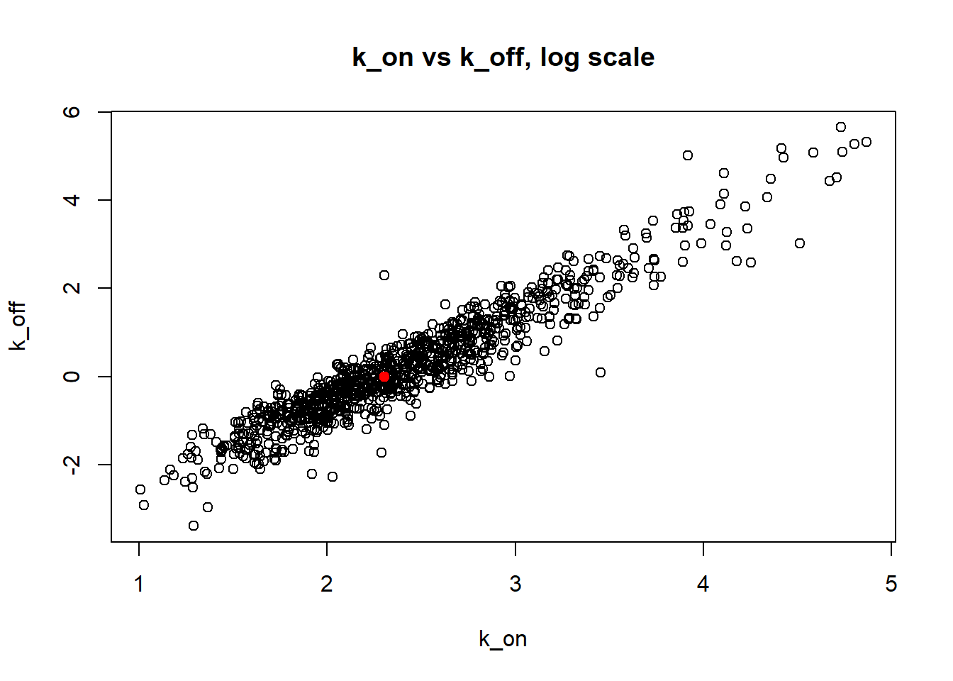
Small value of \(k_{off}\) and big \(k_{on}\) produces a population of cells where majority of observation have high expression level with some quantity oflowly expressed cells (we see it as a long left tail on the distribution graph). Even though the population is not clearly separated as in case I (small \(k_{on}/k_{off}\)), we still are able to correctly estimate parameters by MLE method. The solution is not perfect, as we still see some overestimation of parameters on the histogramm, but the meadian is quite close to the true value.
Ref. https://www.nature.com/articles/s41586-018-0836-1
sessionInfo()R version 3.5.0 (2018-04-23)
Platform: x86_64-w64-mingw32/x64 (64-bit)
Running under: Windows 10 x64 (build 17763)
Matrix products: default
locale:
[1] LC_COLLATE=English_United States.1252
[2] LC_CTYPE=English_United States.1252
[3] LC_MONETARY=English_United States.1252
[4] LC_NUMERIC=C
[5] LC_TIME=English_United States.1252
attached base packages:
[1] stats graphics grDevices utils datasets methods base
other attached packages:
[1] robustbase_0.93-3 reticulate_1.13
loaded via a namespace (and not attached):
[1] Rcpp_1.0.2 knitr_1.20 magrittr_1.5 workflowr_1.5.0
[5] lattice_0.20-38 R6_2.3.0 stringr_1.3.1 highr_0.7
[9] tools_3.5.0 grid_3.5.0 git2r_0.26.1 htmltools_0.3.6
[13] yaml_2.2.0 rprojroot_1.3-2 digest_0.6.17 Matrix_1.2-14
[17] later_0.8.0 fs_1.3.1 promises_1.0.1 glue_1.3.0
[21] evaluate_0.11 rmarkdown_1.10 stringi_1.1.7 DEoptimR_1.0-8
[25] compiler_3.5.0 backports_1.1.2 jsonlite_1.5 httpuv_1.5.1