MLE_bootstrap_variability_by_sample_size
Margarita Orlova
December 19, 2019
Last updated: 2020-02-01
Checks: 6 1
Knit directory: Thesis_single_RNA/
This reproducible R Markdown analysis was created with workflowr (version 1.5.0). The Checks tab describes the reproducibility checks that were applied when the results were created. The Past versions tab lists the development history.
Great! Since the R Markdown file has been committed to the Git repository, you know the exact version of the code that produced these results.
Great job! The global environment was empty. Objects defined in the global environment can affect the analysis in your R Markdown file in unknown ways. For reproduciblity it’s best to always run the code in an empty environment.
The command set.seed(20191113) was run prior to running the code in the R Markdown file. Setting a seed ensures that any results that rely on randomness, e.g. subsampling or permutations, are reproducible.
Great job! Recording the operating system, R version, and package versions is critical for reproducibility.
Nice! There were no cached chunks for this analysis, so you can be confident that you successfully produced the results during this run.
Using absolute paths to the files within your workflowr project makes it difficult for you and others to run your code on a different machine. Change the absolute path(s) below to the suggested relative path(s) to make your code more reproducible.
| absolute | relative |
|---|---|
| C:/Users/Moonkin/Documents/GitHub/Thesis_single_RNA/analysis/MLE.py | analysis/MLE.py |
Great! You are using Git for version control. Tracking code development and connecting the code version to the results is critical for reproducibility. The version displayed above was the version of the Git repository at the time these results were generated.
Note that you need to be careful to ensure that all relevant files for the analysis have been committed to Git prior to generating the results (you can use wflow_publish or wflow_git_commit). workflowr only checks the R Markdown file, but you know if there are other scripts or data files that it depends on. Below is the status of the Git repository when the results were generated:
Ignored files:
    Ignored:    .RData
    Ignored:    .Rhistory
    Ignored:    analysis/.RData
    Ignored:    analysis/.Rhistory

Unstaged changes:
    Modified:   Data_sim.Rmd
    Modified:   analysis/MLE_estimation_with_noise_parameter.Rmd
    Modified:   analysis/MLE_variability_by_sample_size.Rmd
    Modified:   analysis/Real_data_filter.Rmd
Note that any generated files, e.g. HTML, png, CSS, etc., are not included in this status report because it is ok for generated content to have uncommitted changes.
There are no past versions. Publish this analysis with wflow_publish() to start tracking its development.
Warning: package 'reticulate' was built under R version 3.5.3Warning: package 'plotrix' was built under R version 3.5.3Warning: package 'vioplot' was built under R version 3.5.3Loading required package: smWarning: package 'sm' was built under R version 3.5.3Package 'sm', version 2.2-5.6: type help(sm) for summary informationLoading required package: zooWarning: package 'zoo' was built under R version 3.5.3
Attaching package: 'zoo'The following objects are masked from 'package:base':
as.Date, as.Date.numericThis section is the continuation of bootstrap MLE estimates variability exploration. This time we would want to know the MLE bootstrap variability as function of sample size.
For each of the \(k_on\), \(k_off\), \(k_r\) case we generate a dataset of 100,200,500 and 1000 cells and bootstrap the data 500 times to estimate parameters with MLE. Then we take a look at boxplot of MLE estimates and the standart deviation by sample size.
All plot below are in log scale.
bootstrap<-function(boot_number,k_on,k_off,kr,n_cells){
  #The function takes k_on,k_off,kr parameters as well as n_cells (number of cells) as input to generate once and then bootstrap it boot_number times. During each iteration of bootstrapping,  calculate MLE estimation for k_on,k_off,kr and store it in i'th row of est matrix
  est=matrix(, nrow = boot_number, ncol = 3)
  x=generate_data(k_on,k_off,kr,n_cells)
  for (i in 1:boot_number){
    boot_x = as.matrix(x[sample(nrow(x),nrow(x),replace=TRUE)])
    est[i,]=MaximumLikelihood(boot_x)}
  return(est)}

MLE_func<-function(boot_number,k_on,k_off,kr,n_cells){
  #Function does bootstrap function for different number of cells (input as a vector) in a loop and stores the result as list of est matrices
  MLE<-list()
  for (i in 1:length(n_cells)){
    est<-bootstrap(boot_number,k_on,k_off,kr,as.integer(n_cells[i]))
    MLE[[i]] <- est}
  return(MLE)}
I) Small \(k_{on}\) and \(k_{off}\) case:
In the case of small \(k_{on}\) and \(k_{off}\), as we saw before, parameters are identifiable so the standart deviation is quite small even for small 100 cell dataset and diminish with the increase of sample size. It is true for \(k_{on}\),\(k_{off}\) and \(k_{r}\) as well.
#True k_on=k_off=0.1
boot_number=500
k_on=as.numeric(0.1)
k_off=as.numeric(0.1)
kr=as.numeric(100)
n_cells<-c(100,200,500,1000)
MLE<-MLE_func(boot_number,k_on,k_off,kr,n_cells)
x1 <- MLE[[1]]
x2 <- MLE[[2]]
x3 <- MLE[[3]]
x4 <- MLE[[4]]
boxplot(log(x1[,1]),log(x2[,1]),log(x3[,1]),log(x4[,1]),xlab="Number of cells",names=c("100", "200","500", "1000"),main="k_on MLE bootstrap, true k_on=0.1")
abline(h = log(0.1),col="red")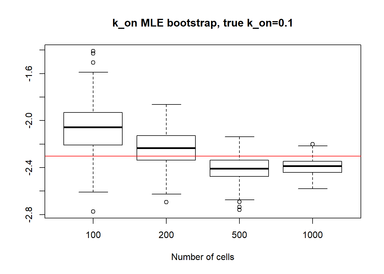
paste("K_on standart deviations:","n=100:",round(sqrt(var(x1[,1],na.rm=TRUE)),3), "; n=200:",round(sqrt(var(x2[,1],na.rm=TRUE)),3), "; n=500:", round(sqrt(var(x3[,1],na.rm=TRUE)),3), "; n=1000:",round(sqrt(var(x4[,1],na.rm=TRUE)),3))[1] "K_on standart deviations: n=100: 0.027 ; n=200: 0.016 ; n=500: 0.009 ; n=1000: 0.006"boxplot(log(x1[,2]),log(x2[,2]),log(x3[,2]),log(x4[,2]),xlab="Number of cells",names=c("100", "200","500", "1000"),main="k_off MLE bootstrap, true k_off=0.1")
abline(h = log(0.1),col="red")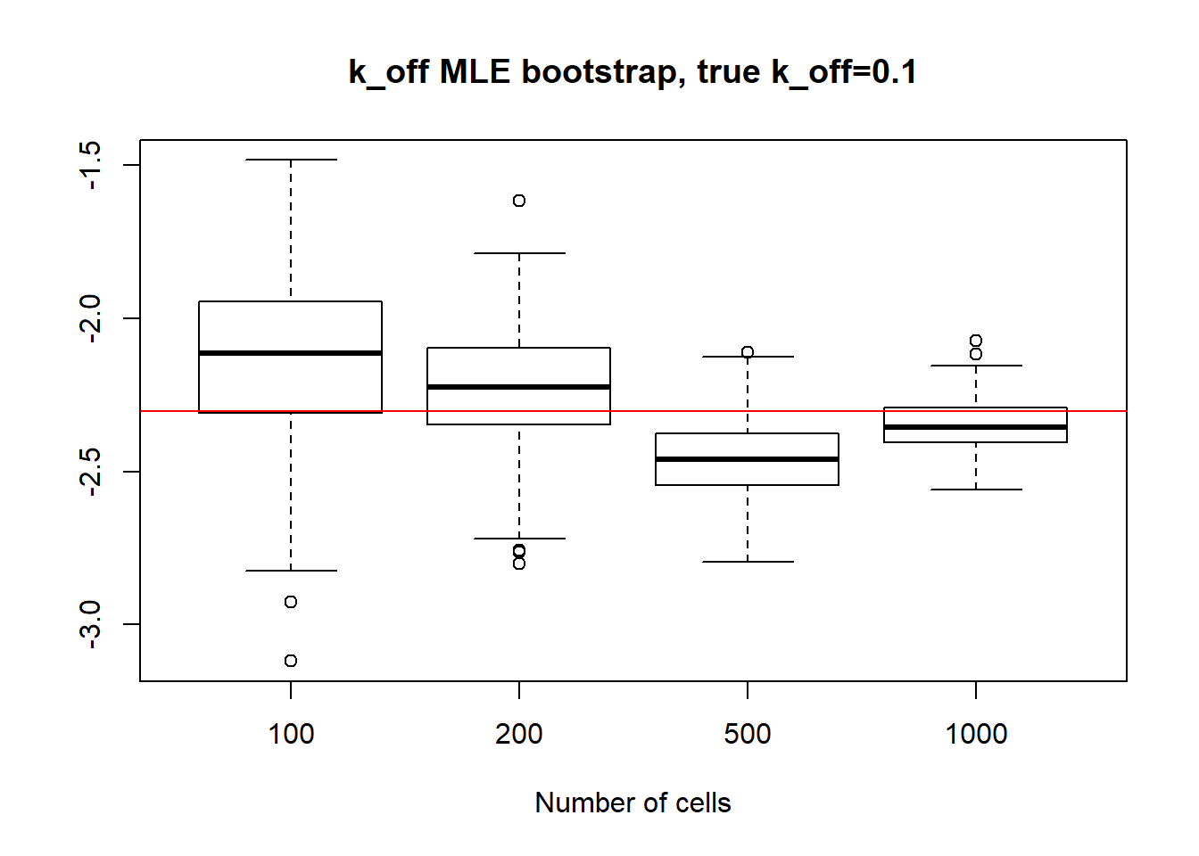
paste("k_off standart deviations:", "n=100:", round(sqrt(var(x1[,2],na.rm=TRUE)),3), "; n=200:",round(sqrt(var(x2[,2],na.rm=TRUE)),3), "; n=500:", round(sqrt(var(x3[,2],na.rm=TRUE)),3), "; n=1000: ", round(sqrt(var(x4[,2],na.rm=TRUE)),3))[1] "k_off standart deviations: n=100: 0.031 ; n=200: 0.02 ; n=500: 0.01 ; n=1000: 0.008"boxplot(log(x1[,3]),log(x2[,3]),log(x3[,3]),log(x4[,3]),xlab="Number of cells",names=c("100", "200","500", "1000"),main="k_r MLE bootstrap, true k_r=100")
abline(h = log(100),col="red")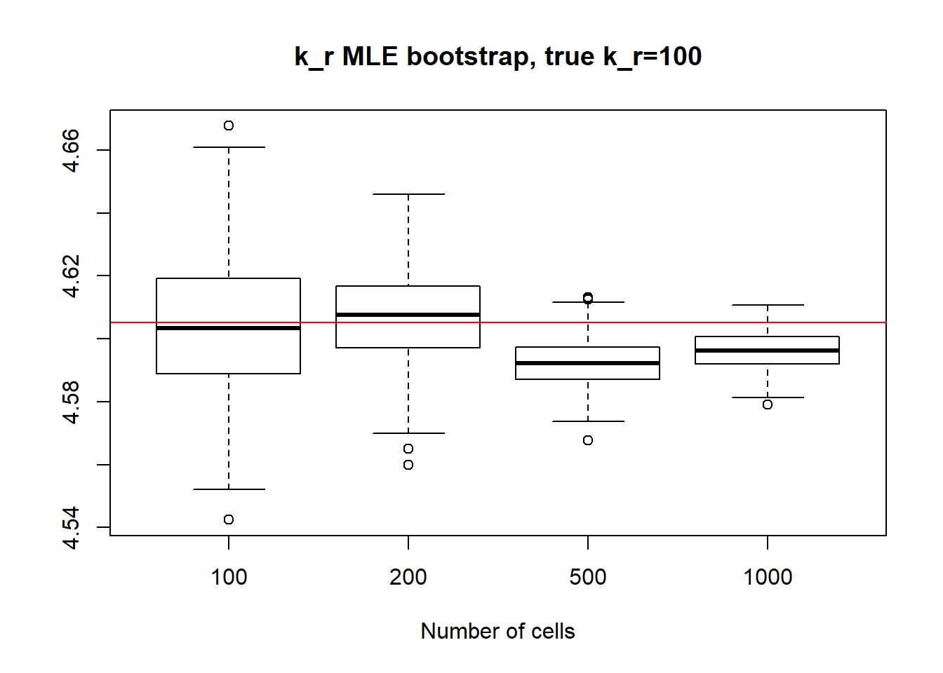
paste("k_r standart deviations:", "n=100:", round(sqrt(var(x1[,3],na.rm=TRUE)),3), "; n=200:",round(sqrt(var(x2[,3],na.rm=TRUE)),3), "; n=500:", round(sqrt(var(x3[,3],na.rm=TRUE)),3), "n=1000:", round(sqrt(var(x4[,3],na.rm=TRUE)),3))[1] "k_r standart deviations: n=100: 2.102 ; n=200: 1.402 ; n=500: 0.77 n=1000: 0.576"II) Large \(k_{on}\) and \(k_{off}\) case:
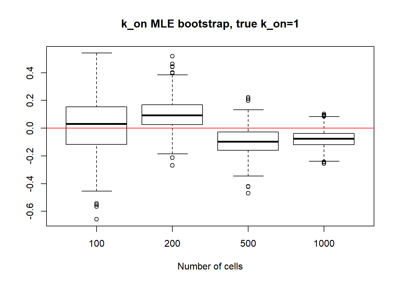
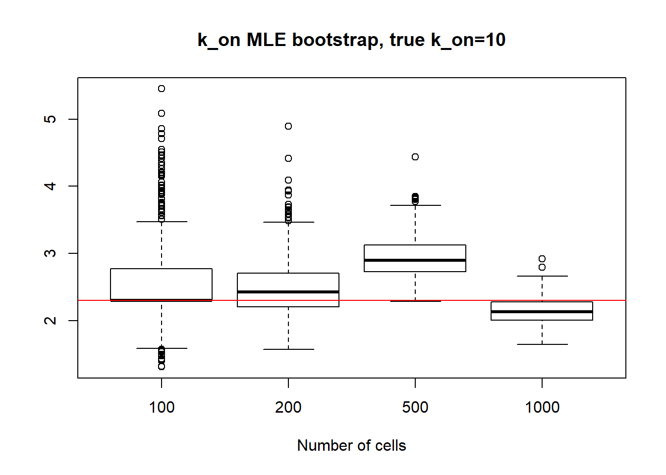
For large \(k_{on}\) and \(k_{off}\) case, we see decrease in standart deviation, but the magnitude is quite high.
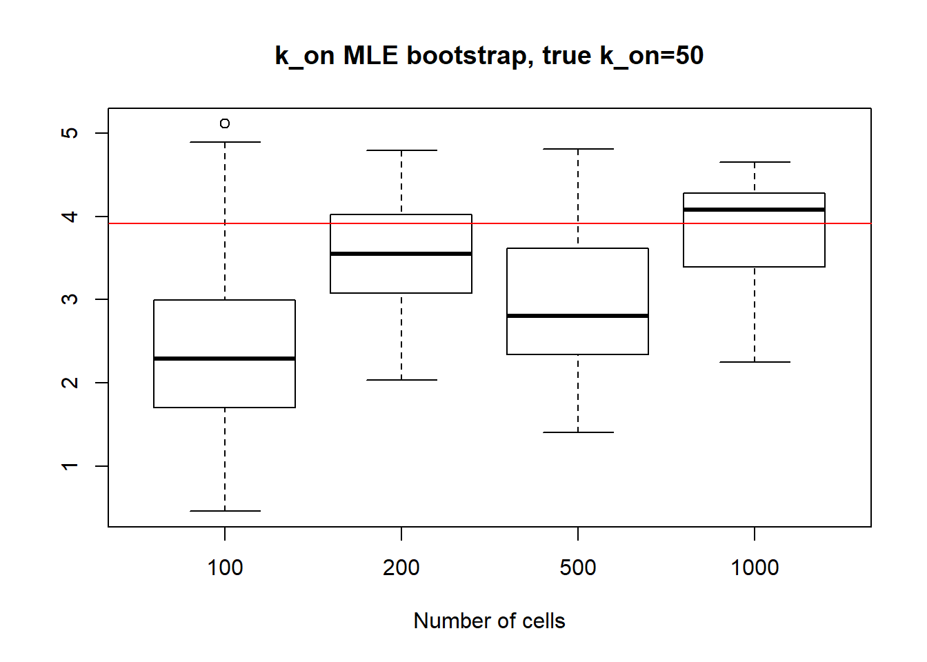
[1] "K_on standart deviations: n=100: 24.888 ; n=200: 20.778 ; n=500: 26.62 ; n=1000: 23.83"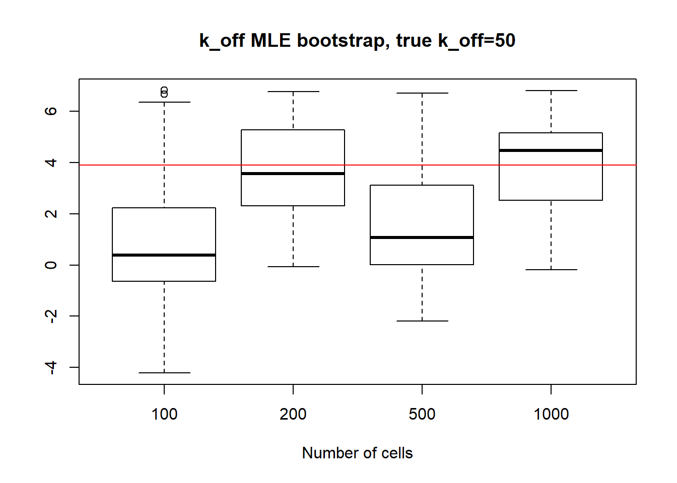
[1] "k_off standart deviations: n=100: 109.668 ; n=200: 145.762 ; n=500: 89.291 ; n=1000: 126.325"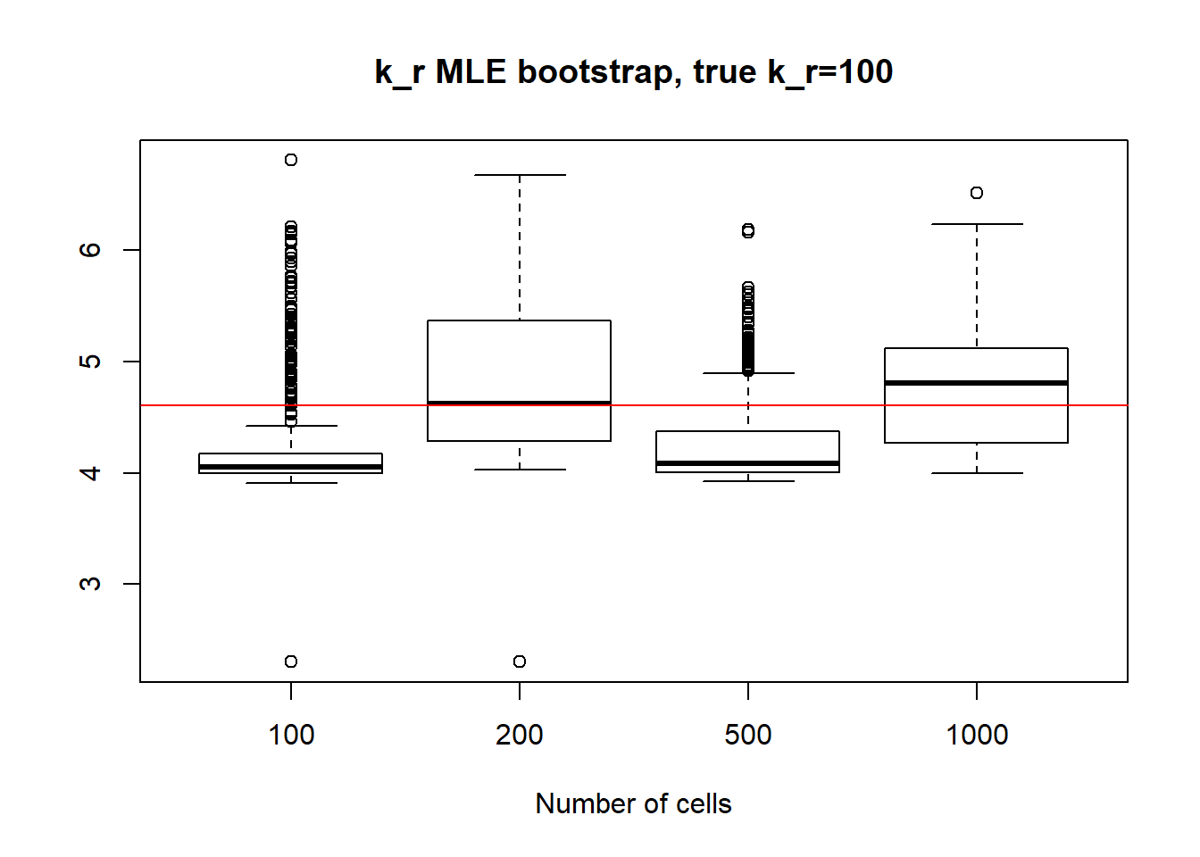
[1] "k_r standart deviations: n=100: 83.034 ; n=200: 112.558 ; n=500: 50.253 n=1000: 74.187"III) Large value of \(k_{off}\) and small \(k_{on}\) case:
For small \(k_{on}\) large \(k_{off}\) we observe that as \(k_{on}\) has small deviation and as we might remember from previous vignette, this is the only identifiable parameter in this scenario. Both \(k_{off}\) and \(k_{r}\) were unidentifiable, so we see high standart deviation even with big data size. We also experience some instability in standart deviation - sample size dependance as we sometimes see increase in standart deviation despite the sample size growth.
[1] "K_on standart deviations: n=100: 0.205 ; n=200: 0.132 ; n=500: 0.093 ; n=1000: 0.06"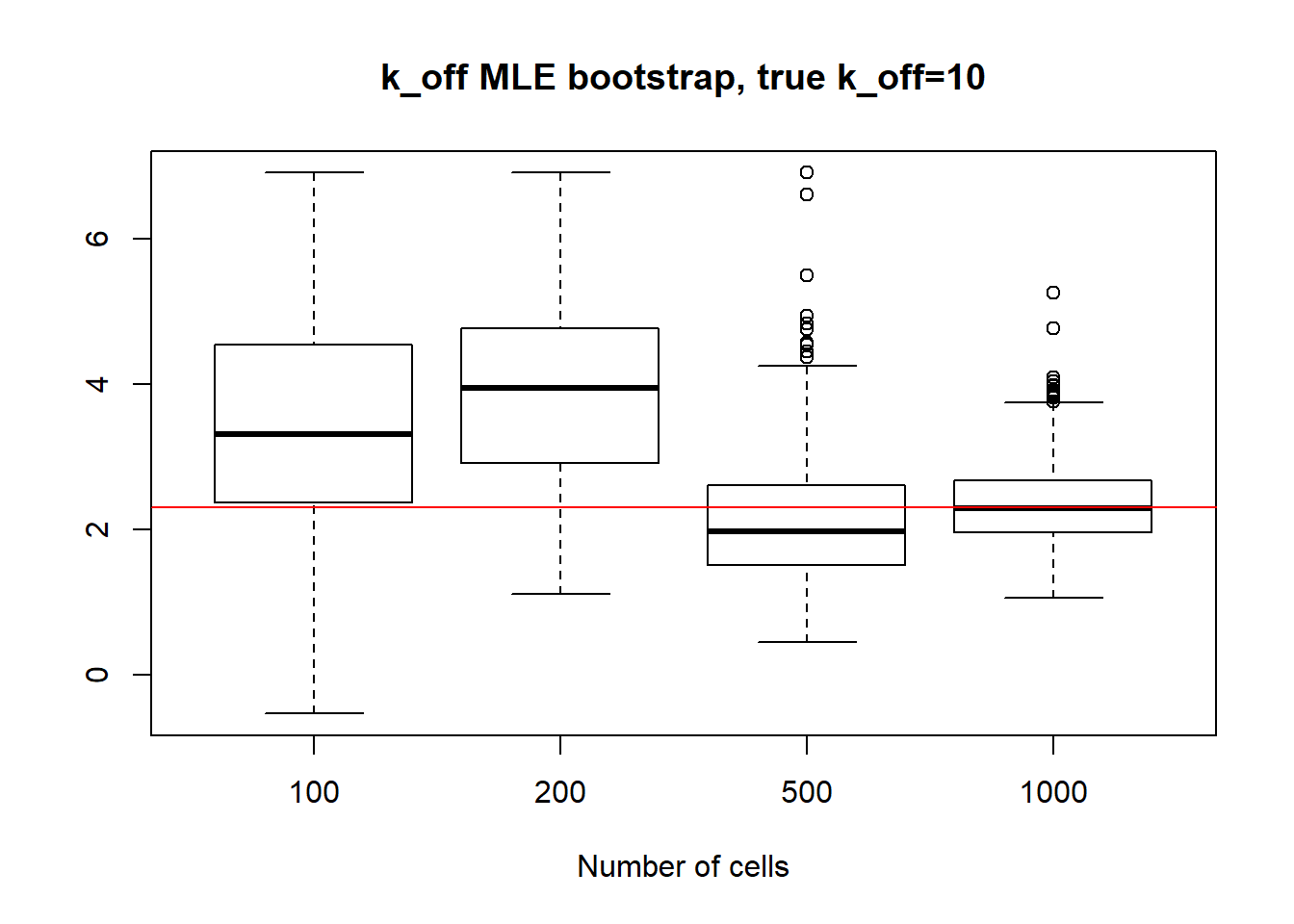
[1] "k_off standart deviations: n=100: 160.242 ; n=200: 139.272 ; n=500: 57.805 ; n=1000: 12.559"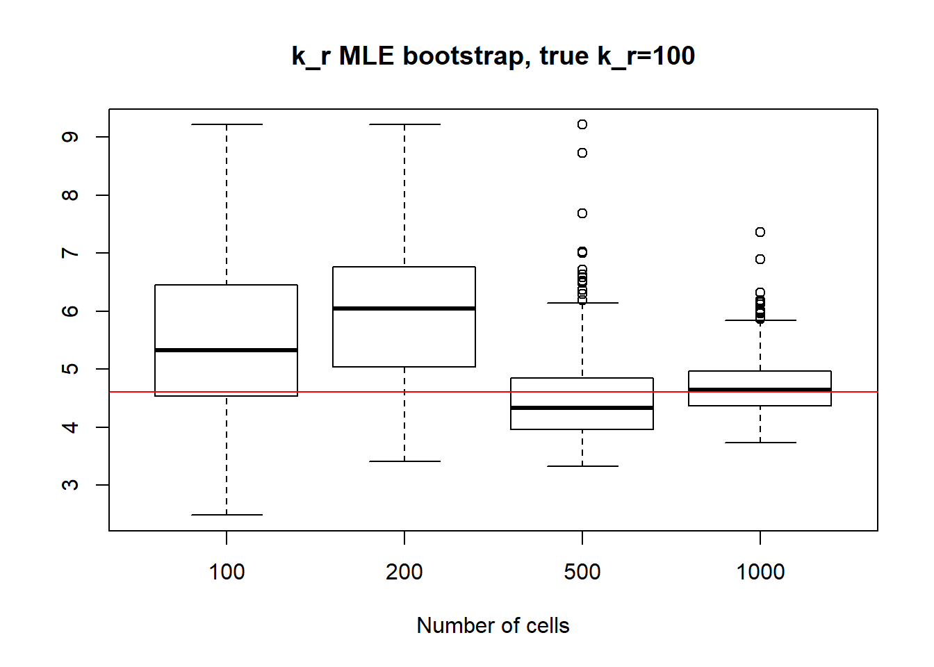
[1] "k_r standart deviations: n=100: 1328.824 ; n=200: 1055.969 ; n=500: 539.731 n=1000: 103.627"IV) Small value of \(k_{off}\) and big \(k_{on}\)
Small value if \(k_{off}\) and big \(k_{on}\) scenario has identifiable parameters, so alike with small value \(k_{on}\), \(k_{on}\) case we observe reasonable standart deviation values, especially for bigger dataset as well as decrease in standart deviation size.
[1] "K_on standart deviations: n=100: 20.615 ; n=200: 9.718 ; n=500: 7.171 ; n=1000: 1.664"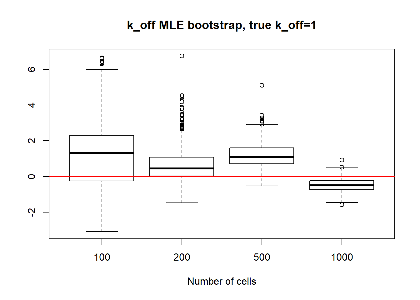
[1] "k_off standart deviations: n=100: 72.209 ; n=200: 38.885 ; n=500: 7.987 ; n=1000: 0.257"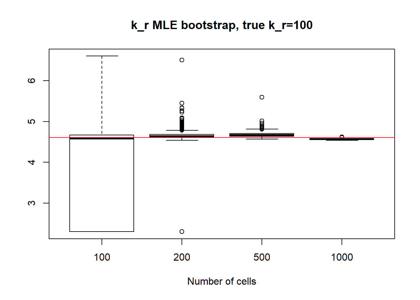
[1] "k_r standart deviations: n=100: 80.019 ; n=200: 32.034 ; n=500: 9.794 n=1000: 1.38"
sessionInfo()R version 3.5.0 (2018-04-23)
Platform: x86_64-w64-mingw32/x64 (64-bit)
Running under: Windows 10 x64 (build 17763)
Matrix products: default
locale:
[1] LC_COLLATE=English_United States.1252
[2] LC_CTYPE=English_United States.1252
[3] LC_MONETARY=English_United States.1252
[4] LC_NUMERIC=C
[5] LC_TIME=English_United States.1252
attached base packages:
[1] stats graphics grDevices utils datasets methods base
other attached packages:
[1] vioplot_0.3.4 zoo_1.8-6 sm_2.2-5.6 plotrix_3.7-5
[5] reticulate_1.13
loaded via a namespace (and not attached):
[1] Rcpp_1.0.2 knitr_1.20 magrittr_1.5 workflowr_1.5.0
[5] lattice_0.20-38 R6_2.3.0 stringr_1.3.1 highr_0.7
[9] tcltk_3.5.0 tools_3.5.0 grid_3.5.0 git2r_0.26.1
[13] htmltools_0.3.6 yaml_2.2.0 rprojroot_1.3-2 digest_0.6.17
[17] Matrix_1.2-14 later_0.8.0 fs_1.3.1 promises_1.0.1
[21] glue_1.3.0 evaluate_0.11 rmarkdown_1.10 stringi_1.1.7
[25] compiler_3.5.0 backports_1.1.2 jsonlite_1.5 httpuv_1.5.1