MLE_bootstrap
Margarita Orlova
December 4, 2019
Last updated: 2020-02-01
Checks: 6 1
Knit directory: Thesis_single_RNA/
This reproducible R Markdown analysis was created with workflowr (version 1.5.0). The Checks tab describes the reproducibility checks that were applied when the results were created. The Past versions tab lists the development history.
Great! Since the R Markdown file has been committed to the Git repository, you know the exact version of the code that produced these results.
Great job! The global environment was empty. Objects defined in the global environment can affect the analysis in your R Markdown file in unknown ways. For reproduciblity it’s best to always run the code in an empty environment.
The command set.seed(20191113) was run prior to running the code in the R Markdown file. Setting a seed ensures that any results that rely on randomness, e.g. subsampling or permutations, are reproducible.
Great job! Recording the operating system, R version, and package versions is critical for reproducibility.
Nice! There were no cached chunks for this analysis, so you can be confident that you successfully produced the results during this run.
Using absolute paths to the files within your workflowr project makes it difficult for you and others to run your code on a different machine. Change the absolute path(s) below to the suggested relative path(s) to make your code more reproducible.
| absolute | relative |
|---|---|
| C:/Users/Moonkin/Documents/GitHub/Thesis_single_RNA/analysis/MLE.py | analysis/MLE.py |
Great! You are using Git for version control. Tracking code development and connecting the code version to the results is critical for reproducibility. The version displayed above was the version of the Git repository at the time these results were generated.
Note that you need to be careful to ensure that all relevant files for the analysis have been committed to Git prior to generating the results (you can use wflow_publish or wflow_git_commit). workflowr only checks the R Markdown file, but you know if there are other scripts or data files that it depends on. Below is the status of the Git repository when the results were generated:
Ignored files:
    Ignored:    .RData
    Ignored:    .Rhistory
    Ignored:    analysis/.RData
    Ignored:    analysis/.Rhistory

Unstaged changes:
    Modified:   Data_sim.Rmd
    Deleted:    analysis/MLE_bootstrap_variability_by_sample_size.Rmd
    Deleted:    analysis/MLE_estimates.Rmd
    Deleted:    analysis/MLE_estimation_with_noise_parameter.Rmd
    Deleted:    analysis/MLE_variability_by_sample_size.Rmd
    Deleted:    analysis/Real_data_filter.Rmd
Note that any generated files, e.g. HTML, png, CSS, etc., are not included in this status report because it is ok for generated content to have uncommitted changes.
There are no past versions. Publish this analysis with wflow_publish() to start tracking its development.
Warning: package 'reticulate' was built under R version 3.5.3Warning: package 'plotrix' was built under R version 3.5.3Warning: package 'robustbase' was built under R version 3.5.1In previous section we have shown MLE estimates variability for datasets generated with the same parameters. Now we would want to investigate the sampling distribution of MLE using bootsrapp.
Bootstrap procedure:
Generate one time 500 cells with given \(k_{on}\), \(k_{off}\) and \(k_r\) parameters
For 500 iterations, bootstrap the sample with replacement
Estimate parameters by maximum likelihood
bootstrap<-function(boot_number,k_on,k_off,kr,n_cells){
  est=matrix(, nrow = boot_number, ncol = 3)
  x=generate_data(k_on,k_off,kr,n_cells)
  for (i in 1:boot_number){
    boot_x = as.matrix(x[sample(nrow(x),nrow(x),replace=TRUE)])
    est[i,]=MaximumLikelihood(boot_x)}
  return(est)}
I) Small \(k_{on}\) and \(k_{off}\) case:
#True k_on=k_off=0.1
boot_number=500
k_on=as.numeric(0.1)
k_off=as.numeric(0.1)
kr=as.numeric(100)
n_cells=as.integer(500)
est<-bootstrap(boot_number,k_on,k_off,kr,n_cells)

hist(log(est[,1]),breaks=30, main="MLE estimate of k_on parameter,true k_on=0.1")
abline(v=log(0.1),col='red')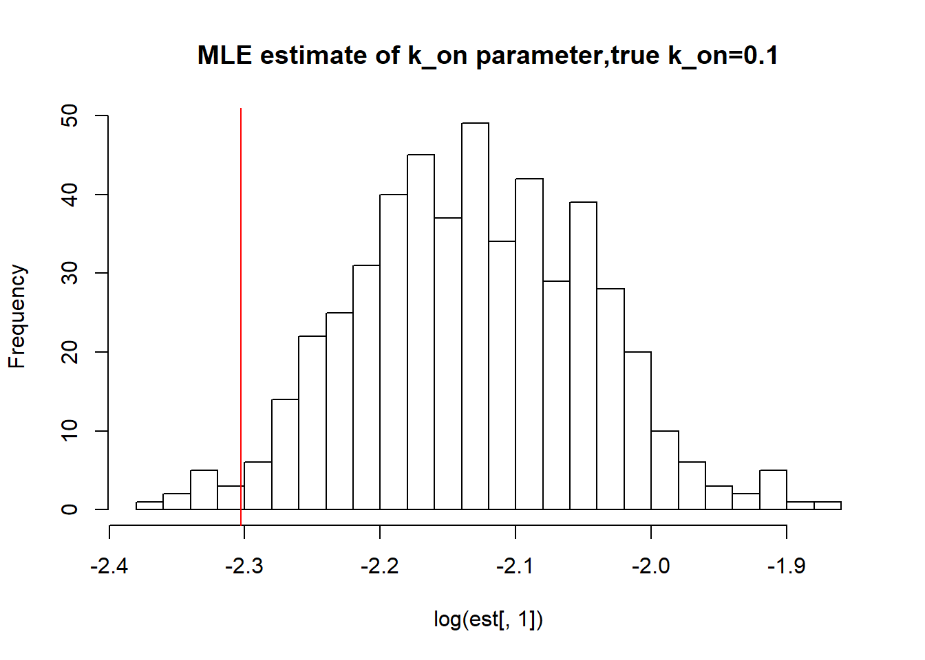
paste("true k_on is 0.1;","k_on mean;",round(mean(est[,1],na.rm=TRUE),3),"k_on median", round(median(est[,1],na.rm=TRUE),3),"k_on st.deviation",round(sqrt(var(est[,1],na.rm=TRUE)),3))[1] "true k_on is 0.1; k_on mean; 0.119 k_on median 0.119 k_on st.deviation 0.01"hist(log(est[,2]),breaks=30, main="MLE estimate of k_off parameter, true k_off=0.1")
abline(v=log(0.1),col='red')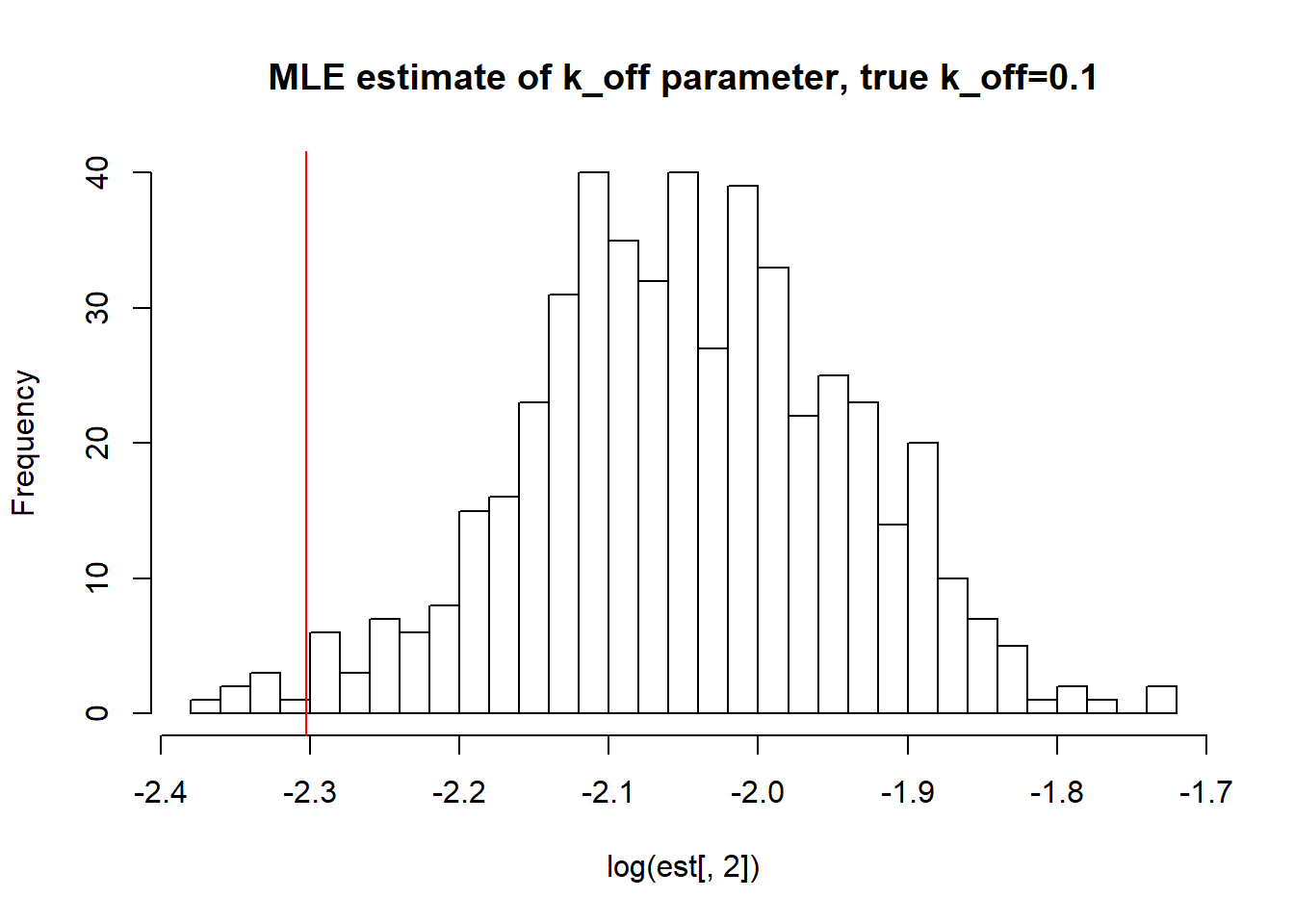
paste("true k_off is 0.1;","k_off mean;",round(mean(est[,2],na.rm=TRUE),3),"k_off median", round(median(est[,2],na.rm=TRUE),3),"k_off st.deviation",round(sqrt(var(est[,2],na.rm=TRUE)),3))[1] "true k_off is 0.1; k_off mean; 0.13 k_off median 0.129 k_off st.deviation 0.014"hist(log(est[,3]),breaks=30, main="MLE estimate of k_r parameter,true k_r=100")
abline(v=log(100),col='red')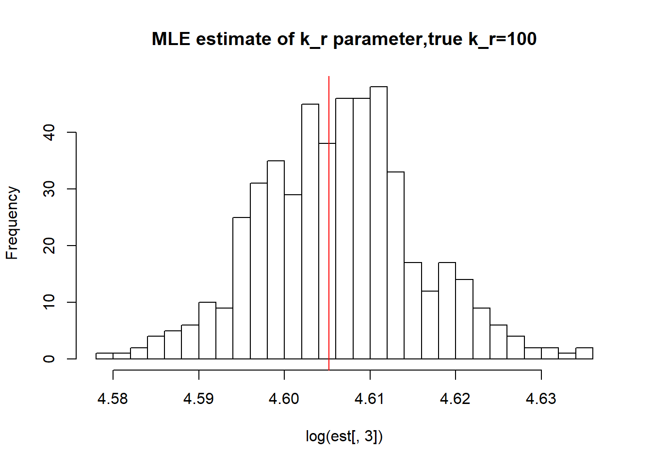
paste("true k_r is 100;","k_r mean;",round(mean(est[,3],na.rm=TRUE),3),"k_r median", round(median(est[,3],na.rm=TRUE),3),"k_r st.deviation",round(sqrt(var(est[,3],na.rm=TRUE)),3))[1] "true k_r is 100; k_r mean; 100.114 k_r median 100.115 k_r st.deviation 0.93"As we saw in previous vignette, this small \(k_{on}\), \(k_{off}\) scenario has clearly identifiable solutions which is confirmed by boorstrap as we see again mean, median are close to the true value and standart deviation is small as well.
II) Large \(k_{on}\) and \(k_{off}\) case:
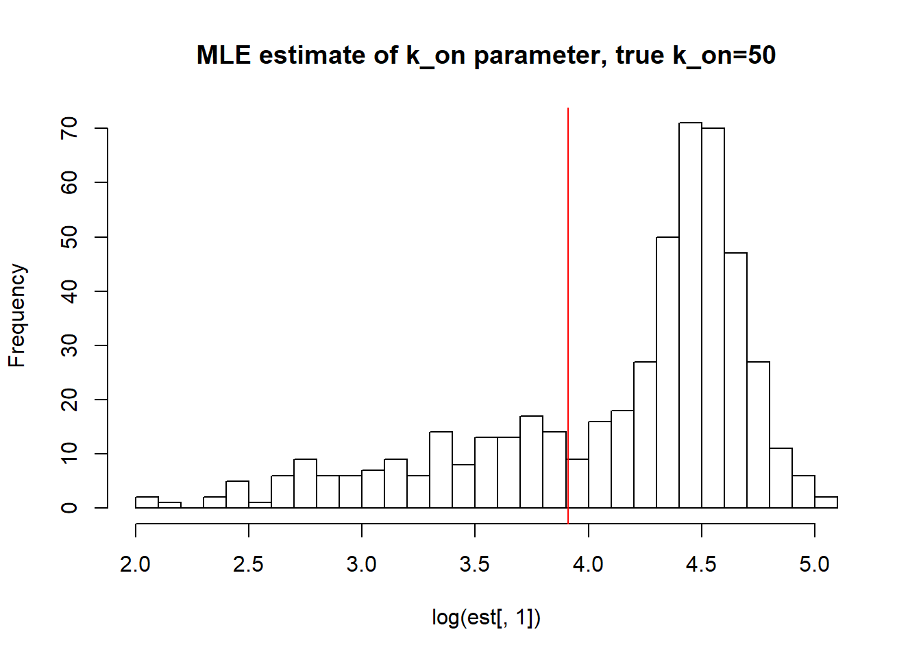
[1] "true k_on is 50; k_on mean; 72.132 k_on median 79.435 k_on st.deviation 32.035"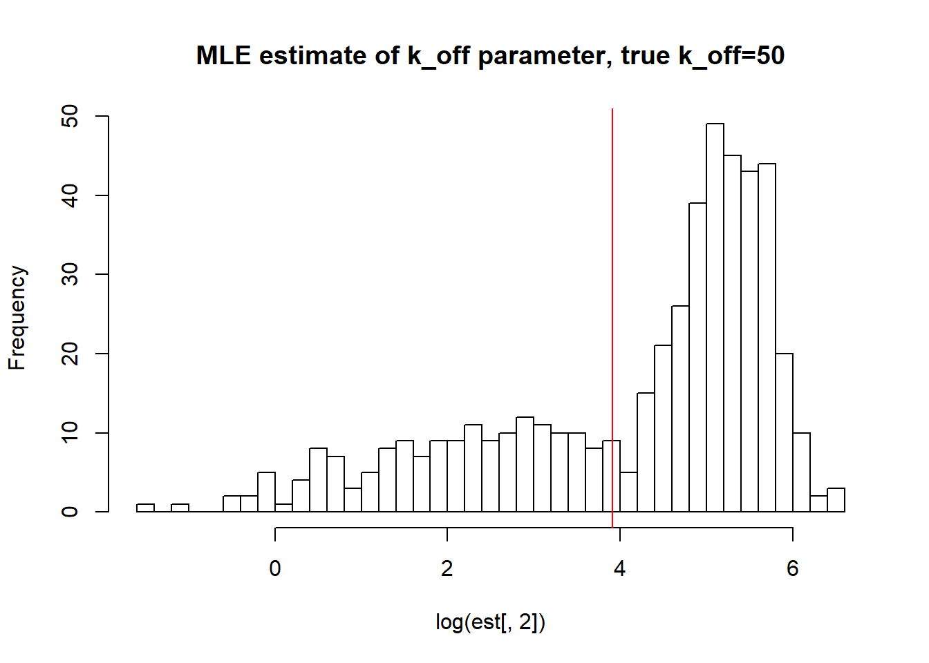
[1] "true k_off is 50; k_off mean; 140.46 k_off median 128.02 k_off st.deviation 125.1"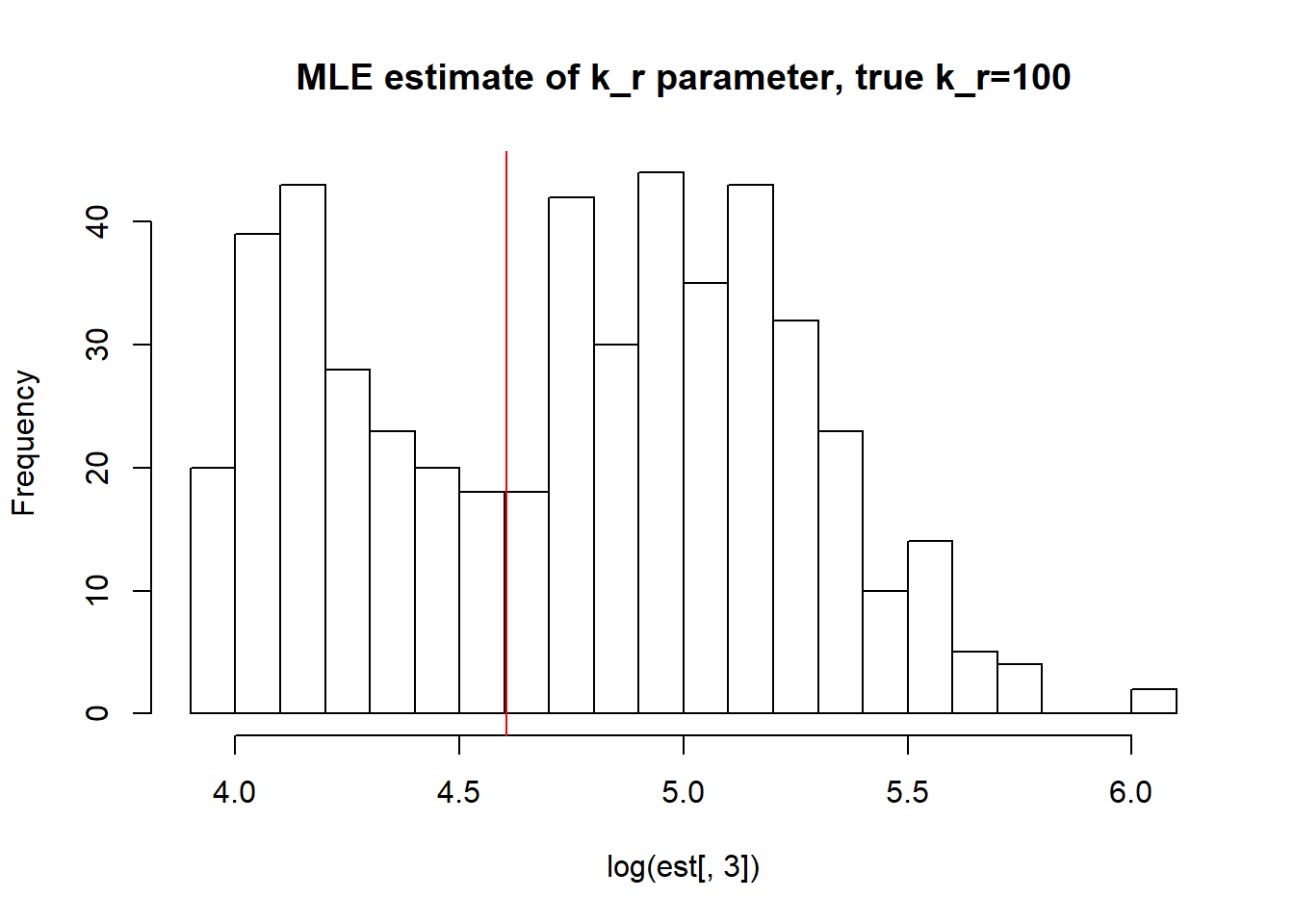
[1] "true k_r is 100; k_r mean; 128.336 k_r median 120.557 k_r st.deviation 62.507"Large \(k_{on}\) and \(k_{off}\) as said earlier produces a dataset with unidentifiable parameters as we do not approach true values with neigher mean or median with huge standart deviation.
III) Large value of \(k_{off}\) and small \(k_{on}\) case:
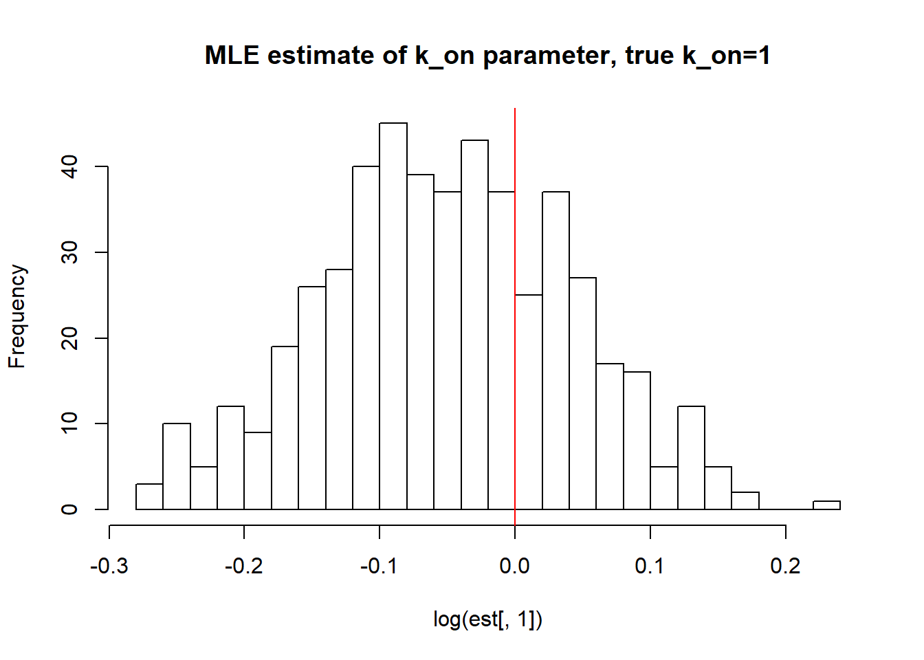
[1] "true k_on is 1; k_on mean; 0.954 k_on median 0.951 k_on st.deviation 0.088"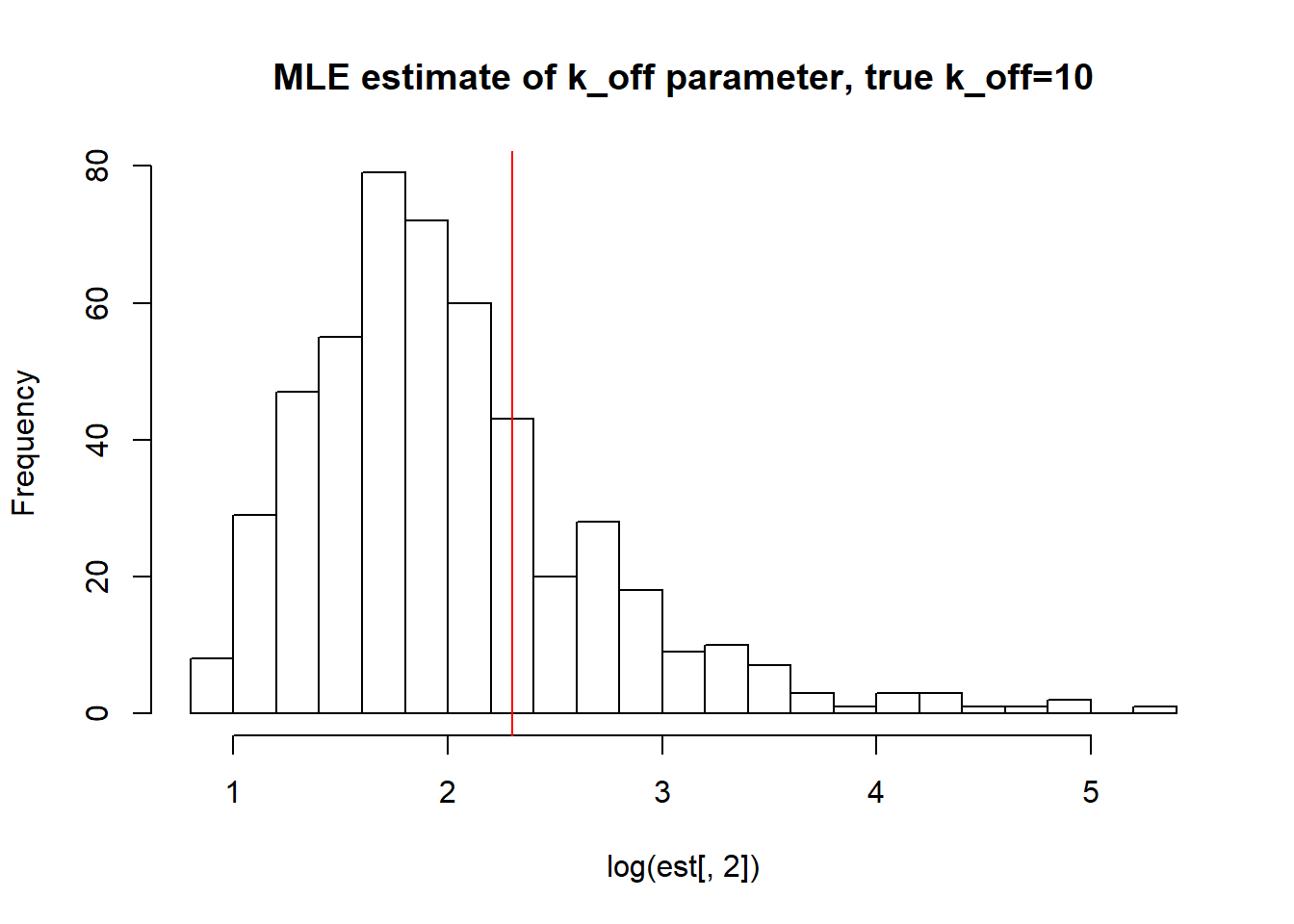
[1] "true k_off is 10; k_off mean; 10.538 k_off median 6.585 k_off st.deviation 15.538"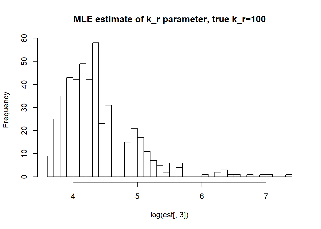
[1] "true k_r is 100; k_r mean; 106.493 k_r median 74.295 k_r st.deviation 127.793"Big \(k_{off}\) and small \(k_{on}\) values allow us to identify \(k_{on}\) parameter, but prevent correct estimation of \(k_{off}\) and \(k_{r}\). We see high standart deviation of the parameters as well as some huge outliers.
IV) Small value of \(k_{off}\) and big \(k_{on}\)
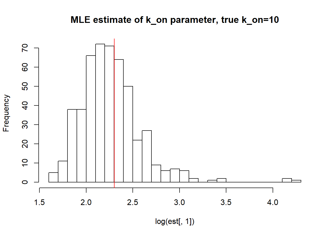
[1] "true k_on is 10; k_on mean; 10.326 k_on median 9.308 k_on st.deviation 5.637"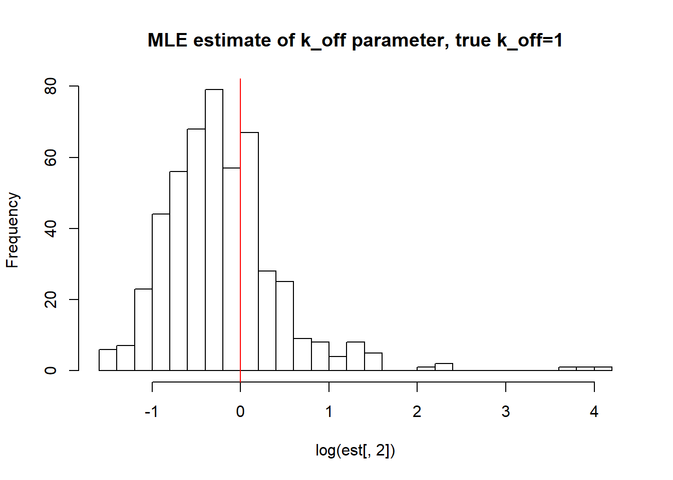
[1] "true k_off is 1; k_off mean; 1.286 k_off median 0.753 k_off st.deviation 3.991"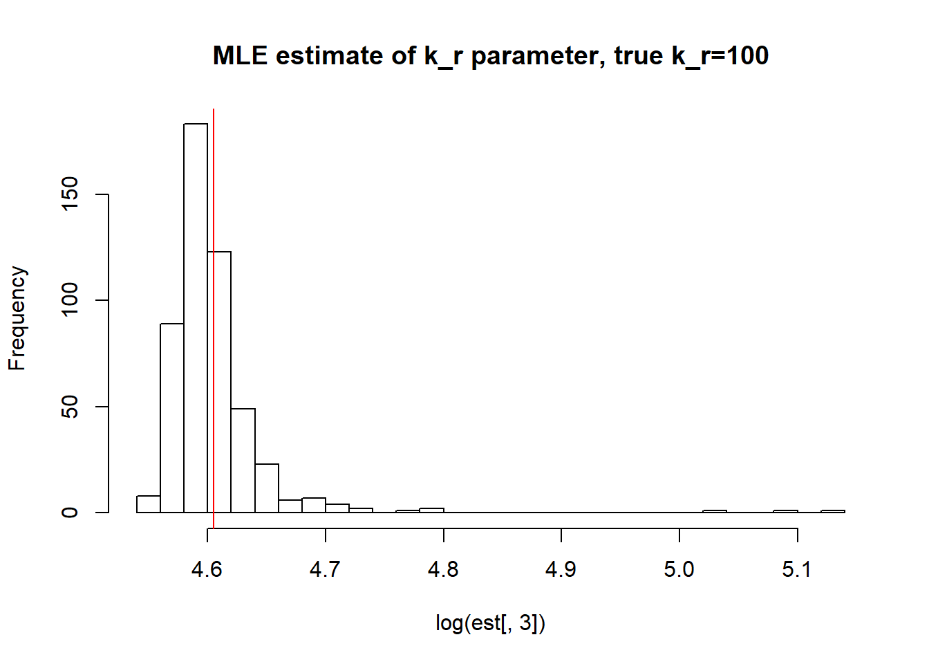
[1] "true k_r is 100; k_r mean; 100.143 k_r median 99.106 k_r st.deviation 5.758"We again observe that parameters get estimated quite accurately, even though not as good as in case I. Standart deviation is reasonable, while mean and median approach true value.
sessionInfo()R version 3.5.0 (2018-04-23)
Platform: x86_64-w64-mingw32/x64 (64-bit)
Running under: Windows 10 x64 (build 17763)
Matrix products: default
locale:
[1] LC_COLLATE=English_United States.1252
[2] LC_CTYPE=English_United States.1252
[3] LC_MONETARY=English_United States.1252
[4] LC_NUMERIC=C
[5] LC_TIME=English_United States.1252
attached base packages:
[1] stats graphics grDevices utils datasets methods base
other attached packages:
[1] robustbase_0.93-3 plotrix_3.7-5 reticulate_1.13
loaded via a namespace (and not attached):
[1] Rcpp_1.0.2 knitr_1.20 magrittr_1.5 workflowr_1.5.0
[5] lattice_0.20-38 R6_2.3.0 stringr_1.3.1 highr_0.7
[9] tools_3.5.0 grid_3.5.0 git2r_0.26.1 htmltools_0.3.6
[13] yaml_2.2.0 rprojroot_1.3-2 digest_0.6.17 Matrix_1.2-14
[17] later_0.8.0 fs_1.3.1 promises_1.0.1 glue_1.3.0
[21] evaluate_0.11 rmarkdown_1.10 stringi_1.1.7 DEoptimR_1.0-8
[25] compiler_3.5.0 backports_1.1.2 jsonlite_1.5 httpuv_1.5.1